Lesson 1. Point aggregation

Aggregation of Cell Towers at country level worldwide

Introduction

In this Lesson, we are going to aggregate a global dataset of Cell Towers at country level. Commonly, the aggregation points-polygons or polygons-points is done using Spatial Join which is incorporated in the common Python library Geopandas for spatial analysis. Geopandas has improved considerably and the aggregation runs quite fast. But, as we are exploring parallelization, we will test the library Dask which is designed to use the computational resources in parallel. Also, there is an integration to Geopandas which is Dask-Geopandas that will be used to compare the time processing with and without parallelization.

This exercise is designed for teaching purposes of Spatial Data Science with High Performance Computing (HPC) at Aalto University. Thanks to the computational resources provided by CSC this exercise was tested in the Puhti supercomputer using Jupyter interactive session.

Objective

To compare the time processing of a spatial join at a global level using Geopandas and Dask-Geopandas

Datasets

Cell Towers from OpenCellID

The database of Cell Towers was downloaded from OpenCellID and stored in Allas for your availability. The compressed file is ~1 GB and decompressed is ~5 GB. You will download it directly on your supercomputer.

Country admin level

The country border layer was downloaded from Natural Earth and stored in Allas for your availability. The Geopackage file is ~4 MB.

Output

The process will give as output the Cell Towers with a country name attribute and also the country border with the aggregation value.

HPC resources

CSC Machine-Puhti:

• Partition: small

• CPU Cores: 8

• Memory (GB): 64

• Local Disk (GB): 400

Download dataset from Allas

The dataset for this practice are stored in Allas and can be downloaded to your local HPC using the next commands. Simply, run the next cells.

!wget -N https://a3s.fi/swift/v1/AUTH_a6b8530017f34af9861fcf45a738ad3f/L2-CellTowers/L2-CellTowers-data.csv.gz

--2024-01-16 11:17:44--  https://a3s.fi/swift/v1/AUTH_a6b8530017f34af9861fcf45a738ad3f/L2-CellTowers/L2-CellTowers-data.csv.gz
Resolving a3s.fi (a3s.fi)... 86.50.254.18, 86.50.254.19
Connecting to a3s.fi (a3s.fi)|86.50.254.18|:443... connected.
HTTP request sent, awaiting response... 304 Not Modified
File ‘L2-CellTowers-data.csv.gz’ not modified on server. Omitting download.

!wget -N https://a3s.fi/swift/v1/AUTH_a6b8530017f34af9861fcf45a738ad3f/L2-CellTowers/L2-CountryAdmin-data.gpkg

--2024-01-16 11:17:45--  https://a3s.fi/swift/v1/AUTH_a6b8530017f34af9861fcf45a738ad3f/L2-CellTowers/L2-CountryAdmin-data.gpkg
Resolving a3s.fi (a3s.fi)... 86.50.254.19, 86.50.254.18
Connecting to a3s.fi (a3s.fi)|86.50.254.19|:443... connected.
HTTP request sent, awaiting response... 304 Not Modified
File ‘L2-CountryAdmin-data.gpkg’ not modified on server. Omitting download.

Hands-on coding

Follow the instructions and run every cell in the supercomputer.

Importing Python libraries

Be sure that you have installed the dask_geopandas in your environment. Get familiar with this library reading a bit the Dask-Geopandas Documentation

import os

# -- for GIS
import pandas as pd
import geopandas as gpd
import dask_geopandas as geodask
import dask
import pyarrow
import numpy as np

# -- for Visualization
import matplotlib.pyplot as plt
import pydeck
import datashader as ds
import datashader.transfer_functions as ds_function
from datashader.utils import export_image
from functools import partial
import colorcet as cc

import time
import warnings
warnings.simplefilter("ignore")

/PUHTI_TYKKY_ibMrDtm/miniconda/envs/env1/lib/python3.10/site-packages/dask/dataframe/_pyarrow_compat.py:17: FutureWarning: Minimal version of pyarrow will soon be increased to 14.0.1. You are using 13.0.0. Please consider upgrading.
  warnings.warn(

# results folder
if not os.path.exists('output'):
    os.makedirs('output')

Read country layer

We will use the country’s administrative border for the Spatial Join. Beforehand, we do a test using a single country with the spatial operation within.

# read country layer
world_admin = gpd.read_file('L2-CountryAdmin-data.gpkg')

# clean and get needed columns
world_admin = world_admin.dropna()

world_gdf = world_admin[['iso3', 'name', 'continent', 'geometry']]

world_gdf.head()

	iso3	name	continent	geometry
0	UGA	Uganda	Africa	MULTIPOLYGON (((33.92110 -1.00194, 33.92027 -1...
1	UZB	Uzbekistan	Asia	MULTIPOLYGON (((70.97081 42.25467, 70.98054 42...
2	IRL	Ireland	Europe	MULTIPOLYGON (((-9.97014 54.02083, -9.93833 53...
3	ERI	Eritrea	Africa	MULTIPOLYGON (((40.13583 15.75250, 40.12861 15...
5	MNG	Mongolia	Asia	MULTIPOLYGON (((116.71138 49.83047, 116.64665 ...

Country visualization

We will create a global view of the countries using Pydeck with interactivity.

# add continent color
cc_admin = {'Africa':[12, 213, 204], 
            'Asia':[221, 76, 8], 
            'Europe':[8, 173, 225], 
            'Americas':[12, 211, 39], 
            'Oceania':[194, 11, 212]
           }

# in a new column
world_gdf['cc_admin'] = world_gdf.continent.apply(lambda x: cc_admin[x])

# add country name
names = gpd.GeoDataFrame()

names["geometry"] = world_gdf.geometry.centroid
names["name"] = world_gdf.name

%%time

# view state pydeck
view_state = pydeck.ViewState(latitude=40, longitude=0, zoom=0)

# set height and width variables
view = pydeck.View(type="_GlobeView", controller=True)#, width=800, height=800)

layers = [
    pydeck.Layer(
                "GeoJsonLayer",
                id="world-admin",
                data=world_gdf,
                stroked=True,
                filled=True,           
				get_fill_color="cc_admin",
                get_line_color=[230, 230, 230],
                line_width_min_pixels=1
                ),
    pydeck.Layer(
                "TextLayer",
                data=names,
                get_position="geometry.coordinates",
                get_size=10,
                get_color=[70, 70, 70],
                get_text="name",
    ),
          ]

deck = pydeck.Deck(
                views=[view],
                initial_view_state=view_state,
                layers=layers,
                map_provider=None,
                # Note that this must be set for the globe to be opaque
                parameters={"cull": True},
            )

# deck.to_html("output/map.html")

CPU times: user 515 ms, sys: 29.2 ms, total: 544 ms
Wall time: 552 ms

deck

Dask-Geopandas Parallelization

Read the Cell Towers

%%time

# read as a dataframe using pandas
data = pd.read_csv('L2-CellTowers-data.csv.gz', 
                      compression='gzip'
                      )

CPU times: user 1min 18s, sys: 7.97 s, total: 1min 26s
Wall time: 1min 30s

# let's check how much memory is it using
memory = data.memory_usage(index=True).sum()

print(f'Total memory used for Cell Towers: {memory/1000000000} GB')

Total memory used for Cell Towers: 5.293554912 GB

data.head()

	radio	mcc	net	area	cell	unit	lon	lat	range	samples	changeable	created	updated	averageSignal
0	UMTS	262	2	801	86355	0	13.285512	52.522202	1000	7	1	1282569574	1300155341	0
1	GSM	262	2	801	1795	0	13.276907	52.525714	5716	9	1	1282569574	1300155341	0
2	GSM	262	2	801	1794	0	13.285064	52.524000	6280	13	1	1282569574	1300796207	0
3	UMTS	262	2	801	211250	0	13.285446	52.521744	1000	3	1	1282569574	1299466955	0
4	UMTS	262	2	801	86353	0	13.293457	52.521515	1000	2	1	1282569574	1291380444	0

%%time 

# create a Geodataframe
geodata = gpd.GeoDataFrame(data, 
                           geometry = gpd.points_from_xy(data.lon, data.lat),
                           crs=4326)

CPU times: user 31 s, sys: 5.61 s, total: 36.6 s
Wall time: 36.7 s

print(f'Total cell towers: {len(geodata)}')

Total cell towers: 47263882

Visualization

To visualize large datasets there are already specialized tools like Pydeck and Datashader/Holoviews. The development of big data formats has advanced to new light extensions of data like Geoparquet from Pyarrow and it is integrated into a new visualization library called Lonboard which is developed for fast and interactive visualization of vector data in Jupyter.

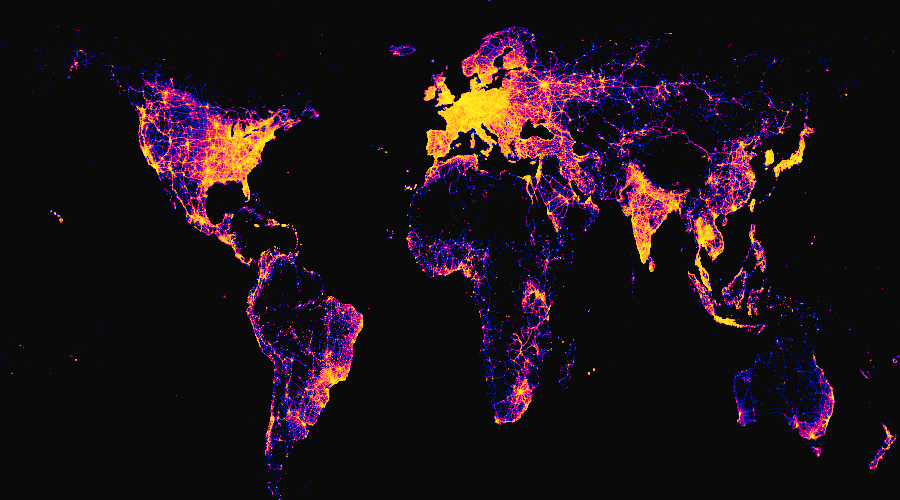
For this example with Cell Towers we are going to explore the options with Datashader.

%%time

# canvas object
canvas = ds.Canvas(plot_width=900, plot_height=500)

# variable columns aggregation like agg=ds.max("column-name")
agg = canvas.points(geodata, geometry='geometry', agg=ds.count())

# image shade with a distribution like ‘eq_hist’ [default], ‘cbrt’ (cube root), ‘log’ (logarithmic), and ‘linear’
# cmaps like fire, kb, kr, kg, bgyw

im = ds_function.shade(agg, cmap=cc.bmy, how="eq_hist")
ds_function.set_background(im, "#0A0A0A")

# save
export = partial(export_image, background = "#0A0A0A", export_path='output')
export(im, 'CellTowers-worldwide')

CPU times: user 2min 16s, sys: 5.01 s, total: 2min 21s
Wall time: 2min 22s

By country

If you want to visualize the Cell Towers by country check the MCC (Mobile Country Code) for example if you want to subset only Finland you can use the MCC=244, or combine codes like Estonia 248, Sweden 240, Denmark 238, Norway 242, India 404, Germany 262, etc

%%time

# -- Choose MCC
MCC = [262]
geodata_view = geodata.loc[geodata.mcc.isin(MCC)]

# canvas object
canvas = ds.Canvas(plot_width=500, plot_height=600)

# variable columns aggregation like agg=ds.max("column-name")
agg = canvas.points(geodata_view, geometry='geometry', agg=ds.count())

# image shade with a distribution like ‘eq_hist’ [default], ‘cbrt’ (cube root), ‘log’ (logarithmic), and ‘linear’
# cmaps like fire, kb, kr, kg, bgyw

im = ds_function.shade(agg, cmap=cc.bgyw, how="eq_hist")
ds_function.set_background(im, "#0A0A0A")

# save
export = partial(export_image, background = "#0A0A0A", export_path='output')
export(im, f'CellTowers-MCC-{MCC}')

CPU times: user 9.02 s, sys: 369 ms, total: 9.39 s
Wall time: 9.41 s

Dask-Dataframe

To create a Dask-Dataframe we need to digest a Geodataframe from Geopandas using the function from_geopandas() and the new table object wil operate efficiently using the Geopandas functions with HPC resources. To make the process efficient Dask uses partitions which refers to Geodataframe indexed into the Dask-Dataframe in this case 16 partitions.

%%time

# antennas to Dask
world_towers = geodask.from_geopandas(geodata, npartitions=16)

CPU times: user 12.8 s, sys: 1.46 s, total: 14.2 s
Wall time: 14.3 s

Computing test

There is a particularity of the Dask-Dataframe. When you want to generate statistics or spatial operations you need to use the function compute() or it will not work. This happens because Dask generates a mapping workflow and it operates once you give the order using compute(). Let’s see some small examples and let’s monitor the HPC usage as well.

To check the resources monitoring you can simply open htop in the terminal of Jupyter Lab. The next image shows that 8 cores are reserved for our process. From 17 to 24

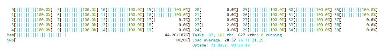
Let’s see some examples of the processing with Dask. Te output will be empty because there is no computation.

%%time

# -- What is the average range of the Cell Towers?

world_towers.range.mean()

CPU times: user 4.03 ms, sys: 4 µs, total: 4.03 ms
Wall time: 4.01 ms

dd.Scalar<series-..., dtype=float64>

Now we will use compute() to generate the value. We will notice that it will operate for a longer time because it is running. While it is running you can notice how the resources are being used in htop.

Cores are operating in parallel from the 17 to the 24.

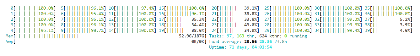
It will give a processed value as output.

%%time 

# using compute
world_towers.range.mean().compute()

CPU times: user 10.6 s, sys: 3.37 s, total: 14 s
Wall time: 7.56 s

2391.7451241732533

Spatial operation test

Let’s do a spatial operation computing the number of points in a selected country. For this example, we will check the points within the ISO3=FIN for Finland.

# get iso3 geometry
iso3_geom = 'FIN'
iso3_country = world_gdf.loc[world_gdf.iso3==iso3_geom].reset_index(drop=True).at[0, 'geometry']

This first process is tested only as a mapping workflow (no processing). You will notice how the output is empty as we have seen before.

%%time
s = time.time()

# -- Test scheduled

# check cell towers within
mcc_within = world_towers.within(iso3_country)

# mask
fin_celltowers = world_towers.loc[mcc_within]

# ---------------------------------------------------------
time_scheduled = time.time() - s

mcc_within

CPU times: user 12 ms, sys: 3 ms, total: 15 ms
Wall time: 16.8 ms

Dask Series Structure:
npartitions=16
0           bool
2953993      ...
            ... 
44309890     ...
47263881     ...
dtype: bool
Dask Name: within, 3 graph layers

Then, we will use compute() to run the mapping workflow scheduled. It will give a processed output.

%%time
s = time.time()

# check cell towers within using compute
mcc_within = world_towers.within(iso3_country).compute()

# mask - Use the Geodataframe because de Dask-Dataframe has partitions and index is not correct
fin_celltowers = geodata.loc[mcc_within]

# ---------------------------------------------------------
time_compute = time.time() - s

mcc_within

CPU times: user 2min 18s, sys: 3.17 s, total: 2min 21s
Wall time: 26.5 s

0           False
1           False
2           False
3           False
4           False
            ...  
47263877    False
47263878    False
47263879    False
47263880    False
47263881    False
Length: 47263882, dtype: bool

type(fin_celltowers)

geopandas.geodataframe.GeoDataFrame

For your information, if you have a Dask-Dataframe object and you want to convert it toa Geodataframe you simply run `Dask-Object.compute()’ and it will give a Geodataframe as an output.

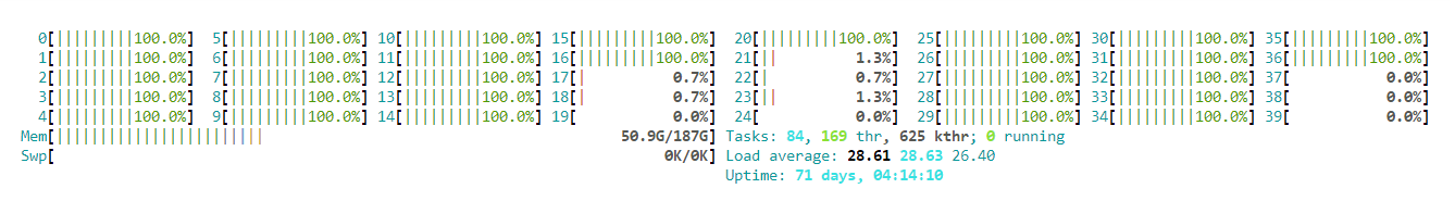
Let’s do the same process using only Geopandas. We will notice in the HPC resources that the Geopandas uses fully a single core.

From our reserved 8 cores, Geopandas uses only the number 20

%%time 
s = time.time()

# check cell towers within using compute
mcc_within_gdf = geodata.within(iso3_country)

# mask
fin_celltowers_gdf = geodata.loc[mcc_within]

# ---------------------------------------------------------
time_gpd = time.time() - s

mcc_within_gdf

CPU times: user 1min 51s, sys: 24.6 ms, total: 1min 51s
Wall time: 1min 51s

0           False
1           False
2           False
3           False
4           False
            ...  
47263877    False
47263878    False
47263879    False
47263880    False
47263881    False
Length: 47263882, dtype: bool

The cell towers we are masking using within() are in the Finland border. Let’s check with Datashader

%%time

# canvas object
canvas = ds.Canvas(plot_width=400, plot_height=600)

# variable columns aggregation like agg=ds.max("column-name")
agg = canvas.points(fin_celltowers_gdf, geometry='geometry', agg=ds.count())

# image shade with a distribution like ‘eq_hist’ [default], ‘cbrt’ (cube root), ‘log’ (logarithmic), and ‘linear’
# cmaps like fire, kb, kr, kg, bgyw

im = ds_function.shade(agg, cmap=cc.kbc, how="eq_hist")
ds_function.set_background(im, "#0A0A0A")

# save
export = partial(export_image, background = "#0A0A0A", export_path='output')
export(im, f'CellTowers-MCC-within-{iso3_geom}')

CPU times: user 771 ms, sys: 13 ms, total: 784 ms
Wall time: 785 ms

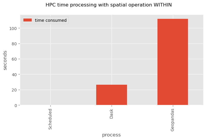
About the performance

As we expected running Dask is faster than Geopandas due to the parallel utilization of Cores.

Here is a quick view of the time process of the within spatial operation.

plt.style.use('ggplot')

# times
time_sub = pd.DataFrame({'process':['Scheduled', 'Dask', 'Geopandas'],
                         'time consumed':[time_scheduled, time_compute, time_gpd]}).set_index('process')

ax = time_sub.plot(figsize=(8, 4), kind='bar');

ax.set_ylabel('seconds')
ax.set_xlabel('process')

plt.suptitle('HPC time processing with spatial operation WITHIN');

Global Spatial Join

We are going to run the Spatial Join to all cell towers worldwide using the country’s administrative border. The comparison will be done using Dask with 8 cores and Geopandas with a single core.

Dask-Parallel

Dask-Geopandas supports only inner operation in Spatial Join and some of the cell towers were removed most probably because they were out of the country polygons.

We will obtain two outputs: 1) Cell Towers with the country attribute, and 2) Country geometry with cell towers count.

%%time

s = time.time()

# ----- Spatial Join with dask

celltowers_dask = geodask.sjoin(world_towers, world_gdf, 
                         predicate='within', how='inner').compute()

# ------------------------------------------- 
time_dask = time.time() - s

CPU times: user 3min 11s, sys: 23.7 s, total: 3min 35s
Wall time: 1min 24s

celltowers_dask.head()

	radio	mcc	net	area	cell	unit	lon	lat	range	samples	changeable	created	updated	averageSignal	geometry	index_right	iso3	name	continent	cc_admin
0	UMTS	262	2	801	86355	0	13.285512	52.522202	1000	7	1	1282569574	1300155341	0	POINT (13.28551 52.52220)	188	DEU	Germany	Europe	[8, 173, 225]
1	GSM	262	2	801	1795	0	13.276907	52.525714	5716	9	1	1282569574	1300155341	0	POINT (13.27691 52.52571)	188	DEU	Germany	Europe	[8, 173, 225]
2	GSM	262	2	801	1794	0	13.285064	52.524000	6280	13	1	1282569574	1300796207	0	POINT (13.28506 52.52400)	188	DEU	Germany	Europe	[8, 173, 225]
3	UMTS	262	2	801	211250	0	13.285446	52.521744	1000	3	1	1282569574	1299466955	0	POINT (13.28545 52.52174)	188	DEU	Germany	Europe	[8, 173, 225]
4	UMTS	262	2	801	86353	0	13.293457	52.521515	1000	2	1	1282569574	1291380444	0	POINT (13.29346 52.52152)	188	DEU	Germany	Europe	[8, 173, 225]

%%time

s = time.time()

# ----- Spatial Aggregation

# count cell towers
celltowers_count = celltowers_dask.groupby('iso3').iso3.agg('count')

# add index
celltowers_iso3 = gpd.GeoDataFrame(index=celltowers_dask.iso3.unique())

# add cell towers count
celltowers_iso3['count'] = celltowers_count

# add iso3
celltowers_iso3 = celltowers_iso3.reset_index(drop=False).rename(columns={'index':'iso3'})

# add geom
celltowers_borders = world_gdf.merge(celltowers_iso3, on='iso3', how='inner')

# ------------------------------------------- 
time_agg = time.time() - s

CPU times: user 2.17 s, sys: 264 ms, total: 2.44 s
Wall time: 2.45 s

celltowers_borders.head()

	iso3	name	continent	geometry	cc_admin	count
0	UGA	Uganda	Africa	MULTIPOLYGON (((33.92110 -1.00194, 33.92027 -1...	[12, 213, 204]	44169
1	UZB	Uzbekistan	Asia	MULTIPOLYGON (((70.97081 42.25467, 70.98054 42...	[221, 76, 8]	23384
2	IRL	Ireland	Europe	MULTIPOLYGON (((-9.97014 54.02083, -9.93833 53...	[8, 173, 225]	142387
3	ERI	Eritrea	Africa	MULTIPOLYGON (((40.13583 15.75250, 40.12861 15...	[12, 213, 204]	110
4	MNG	Mongolia	Asia	MULTIPOLYGON (((116.71138 49.83047, 116.64665 ...	[221, 76, 8]	7990

print(f'Total cell towers before Spatial Join: {len(world_towers)}')
print(f'Total cell towers with Spatial Join in Dask: {len(celltowers_dask)}') 
print(f'Total output countries: {celltowers_dask.name.nunique()}\n')

print(f'Total Spatial Join time Dask: {round(time_dask/60, 2)} minutes')
print(f'Total country aggregation time: {round(time_agg/60, 2)} minutes')

Total cell towers before Spatial Join: 47263882
Total cell towers with Spatial Join in Dask: 45975188
Total output countries: 225

Total Spatial Join time Dask: 1.41 minutes
Total country aggregation time: 0.04 minutes

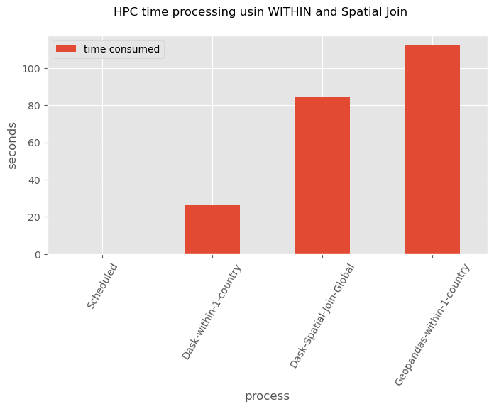
Time processing

In a comparison of Dask and Geopandas we can see that Dask operates faster and uses the HPC resources efficiently. On the other hand, Geopandas takes longer time processing 1 country than Dask processing at global level (225 countries)

plt.style.use('ggplot')

# times
time_sub = pd.DataFrame({'process':['Scheduled', 'Dask-within-1-country',  'Dask-Spatial-Join-Global', 'Geopandas-within-1-country',],
                         'time consumed':[time_scheduled, time_compute, time_dask, time_gpd ]}).set_index('process')

ax = time_sub.plot(figsize=(8, 4), kind='bar');

ax.set_ylabel('seconds')
ax.set_xlabel('process')

plt.xticks(rotation = 60)
plt.suptitle('HPC time processing usin WITHIN and Spatial Join');

Geopandas-single core

Unfortunately, when running the Spatial Join with Geopandas the process runs out of memory. Geopandas uses the memory gradually in the spatial join and when reaching the limit in Puhti it breaks the connection.

If you try you will find a message after the connection breaks.

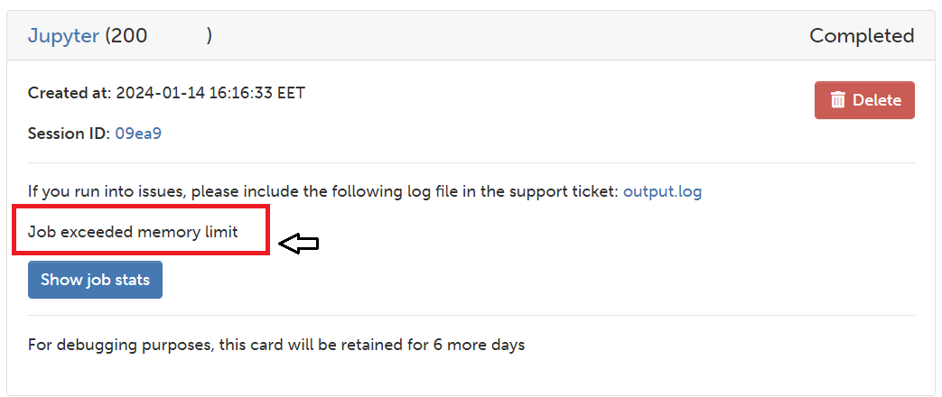
So, it shows how efficiently Dask-Geopandas can operate using parallelization. Sorry, Geopandas.

Note!

If you want to measure the time processing using Geopandas you can operate spatial join in a loop, per country, it will take quite long processing time. This approach was avoid to give a clear and fast view of Parallelization with Dask-Geopandas

Country visualization

Let’s give a quick view to the output of the Spatial Join

# add a category column
celltowers_dask["cat"] = celltowers_dask["iso3"].astype("category")
celltowers_borders["cat"] = celltowers_borders["iso3"].astype("category")

celltowers_dask.dtypes

radio            string[pyarrow]
mcc                        int64
net                        int64
area                       int64
cell                       int64
unit                       int64
lon                      float64
lat                      float64
range                      int64
samples                    int64
changeable                 int64
created                    int64
updated                    int64
averageSignal              int64
geometry                geometry
index_right                int64
iso3             string[pyarrow]
name             string[pyarrow]
continent        string[pyarrow]
cc_admin         string[pyarrow]
cat                     category
dtype: object

%%time

# canvas object
canvas = ds.Canvas(plot_width=900, plot_height=500)

# variable columns aggregation like agg=ds.max("column-name")
agg = canvas.polygons(celltowers_borders, geometry='geometry', agg=ds.max('count'))

# image shade with a distribution like ‘eq_hist’ [default], ‘cbrt’ (cube root), ‘log’ (logarithmic), and ‘linear’
# cmaps like fire, kb, kr, kg, bgyw

im = ds_function.shade(agg, cmap=cc.blues, how='eq_hist')

ds_function.set_background(im, "white")

# save
export = partial(export_image, background = "white", export_path='output')
export(im, 'CellTowers-agg-worldwide-countries')

CPU times: user 4.32 s, sys: 18.2 ms, total: 4.34 s
Wall time: 4.4 s

%%time

# subset of countries
country_names = ['FIN', 'SWE', 'NOR', 'DNK', 'EST', 'LVA', 'LTU', 'DEU', 'POL', 'CZE', 'NLD', 'BEL', 'AUT', 'FRA', 'ESP', 'ITA', 'PRT', 'GBR', 'CHE', 'ISL']
celltowers_cat = celltowers_dask.loc[celltowers_dask['iso3'].isin(country_names)]

# canvas object
canvas = ds.Canvas(plot_width=700, plot_height=800)

# variable columns aggregation like agg=ds.max("column-name")
agg = canvas.points(celltowers_cat, geometry='geometry', agg=ds.count_cat('cat'))

# image shade with a distribution like ‘eq_hist’ [default], ‘cbrt’ (cube root), ‘log’ (logarithmic), and ‘linear’
# cmaps like fire, kb, kr, kg, bgyw
im = ds_function.shade(agg, color_key=cc.glasbey_light)

ds_function.set_background(im, "#0A0A0A")

# save
export = partial(export_image, background = "#0A0A0A", export_path='output')
export(im, 'CellTowers-cat-EU-countries')

CPU times: user 51.1 s, sys: 4.43 s, total: 55.5 s
Wall time: 55.7 s

%%time

# subset of countries
country_names = ['ECU', 'COL', 'PER', 'VEN', 'BRA', 'ARG', 'PRY', 'URY', 'CHL', 'BOL']
celltowers_cat = celltowers_dask.loc[celltowers_dask['iso3'].isin(country_names)]

# canvas object
canvas = ds.Canvas(plot_width=700, plot_height=700)

# variable columns aggregation like agg=ds.max("column-name")
agg = canvas.points(celltowers_cat, geometry='geometry', agg=ds.count_cat('cat'))

# image shade with a distribution like ‘eq_hist’ [default], ‘cbrt’ (cube root), ‘log’ (logarithmic), and ‘linear’
# cmaps like fire, kb, kr, kg, bgyw
im = ds_function.shade(agg, color_key=cc.glasbey_light)

ds_function.set_background(im, "#0A0A0A")

# save
export = partial(export_image, background = "#0A0A0A", export_path='output')
export(im, 'CellTowers-cat-SA-countries')

CPU times: user 14 s, sys: 2.25 s, total: 16.2 s
Wall time: 16.4 s