Lesson 5. OvertureMaps Data

From Local to Global analysis with Arrow

Introduction

In this Lesson, we will fetch Overture Maps data from the local level in Helsinki and the national level of Finland using tags like Buildings and Points of Interest (POI). Then, we will escalate the fetching process at the global level using grids and storing data in parquet format on our local disk (Scratch). The Scratch disk in the Puhti supercomputer has a capacity of 1 Tb which is way bigger than the projappl disk with 50 Gb. So, it is recommended to use the Scratch disk in processes where it is needed to store big amounts of data. We will also explore the compression capacity of Python for big data like PyArrow and cloud formats like GeoParquet. The test done at downloading the entire global data of Overture Maps showed that the data can be kept in only 3.8 GB using 417 GeoParquets.

This exercise is designed for teaching purposes of Spatial Data Science with High Performance Computing (HPC) at Aalto University. Thanks to the computational resources provided by CSC this exercise was tested in the Puhti supercomputer using Jupyter interactive session.

Objective

• To fetch global datasets from Overture Maps using Parallel Computing.

• To analyze global data using GeoParquet and PyArrow. Which main category is the biggest at the global level?

Datasets

Look at the whole data review at Overture Maps Documentation.

Points of Interest

Data with the tag Places contains points of representations of real-world facilities, services, businesses, or amenities. Test done at the global level.

Buildings

Data with the tag Buildings describes human-made structures with roofs or interior spaces that are permanently or semi-permanently in one place (source: OSM building definition). Done locally for Helsinki.

Country Admin Level

• The country border layer was downloaded from Natural Earth and stored in Allas for your availability. The Geopackage file is ~4 MB.

• A low-resolution version was used directly from Geopandas data store.

Capacity

• 2 Cores

• 60 GB memory

• 80 GB disk memory

Output

A workflow that can be used for the analysis of big data at the global level for categorical variables and geo-visualization.

Hands-on coding

Follow the instructions and run every cell in the supercomputer.

Importing Python libraries

Be sure that you have installed the overturemaps-py and lonboard in your environment. Get familiar with this library by reading a bit the lonboard Documentation. Also, be aware that PyArrow and H3Pandas should be in the environment.

For parallelization, we are going to use Dask.

import numpy as np
from shapely.geometry import Polygon
import overturemaps
import geopandas as gpd
import pandas as pd

from IPython.display import IFrame

import gc
import dask_geopandas as geodask
import dask
import pyarrow.parquet as pq

import plotly.express as px
import matplotlib.pyplot as plt
from matplotlib.colors import LogNorm
from palettable.colorbrewer.sequential import Oranges_9, PuRd_9, YlGnBu_9, PuBuGn_9, YlOrRd_9, RdPu_7
from palettable.colorbrewer.qualitative import Paired_12 
from palettable.colorbrewer.diverging import RdYlGn_7, Spectral_9, PiYG_6

from lonboard import Map, PolygonLayer, ScatterplotLayer
from lonboard.colormap import apply_continuous_cmap, apply_categorical_cmap
import pydeck

import h3pandas
import h3

import datashader as ds
import datashader.transfer_functions as ds_function
from datashader.utils import export_image
from functools import partial
import colorcet as cc

import os, shutil, glob
import time
import warnings
warnings.simplefilter("ignore")

# results folder
if not os.path.exists('output'):
    os.makedirs('output')

scratch = '/scratch/project_2009245'

Builings of Helsinki (Local)

Find a Bounding Box

The overture map tool works using a Bounding Box coordinates. You can easily find the coordinates using the online tool Bounding Box Klokantech. You have to select CSV from the dropdown options. We will use a decent area of the Helsinki Region for this initial part.

# bbox coordinates in CSV format
bbox = 24.503673, 60.120966, 25.254511, 60.356827

Materialize data in memory

The overturemaps uses the function overturemaps.record_batch_reader which is an iterator of Arrow. With read_all() we will fetch the data from the AWS S3 Cloud so it might take some minutes.

Let’s get a look to the data types we can fetch using overturemaps.get_all_overture_types()

overturemaps.get_all_overture_types()

['locality',
 'locality_area',
 'administrative_boundary',
 'building',
 'building_part',
 'division',
 'division_area',
 'place',
 'segment',
 'connector',
 'infrastructure',
 'land',
 'land_cover',
 'land_use',
 'water']

%%time

table = overturemaps.record_batch_reader("building", bbox).read_all()

# Temporarily required as of Lonboard 0.8 to avoid a Lonboard bug
# table = table.combine_chunks()

CPU times: user 3.32 s, sys: 902 ms, total: 4.22 s
Wall time: 38.4 s

Let’s take a look at the column names of the Arrow table object. The Arrow Table has a different behavior in comparison of a Pandas Dataframe. If you need to do operation it might have a different sintax than common so it might be good to check the documentation before. For now, we will continue without operations but at we will use them at the global level.

table.column_names

['id',
 'geometry',
 'bbox',
 'version',
 'update_time',
 'sources',
 'subtype',
 'names',
 'class',
 'level',
 'has_parts',
 'height',
 'num_floors',
 'min_height',
 'min_floor',
 'facade_color',
 'facade_material',
 'roof_material',
 'roof_shape',
 'roof_direction',
 'roof_orientation',
 'roof_color',
 'eave_height']

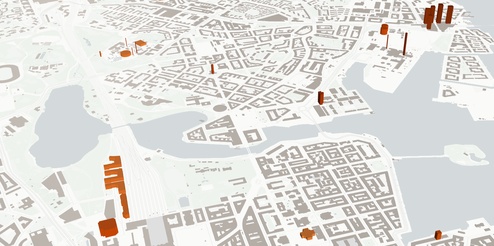
Normalization of building’s height

We will use lonboard to visualize and color the building’s height. Building heights tend to scale non-linearly. That is, most buildings are relatively low, but a few are very tall. So that the low buildings aren’t completely washed out, we’ll use matplotlib’ LogNorm to normalize these values accordingly to a log scale. Take a look at more material in the Lonboard Documentation

# replace height nans in a numpy array
heights = table["height"].to_numpy()
heights = np.nan_to_num(heights, nan=1)

# normalize heights in logarithmic scale
normalizer = LogNorm(1, heights.max(), clip=True)
normalized_heights = normalizer(heights)

Add color palette

You can add color to lonboard to a column with continuous values using apply_continuous_cmap, take a look to the documentation

Let’s add a color from colorbrewer. You can find more options in the documentation but for now, we will use Oranges_9 or PuRd_9.

Oranges_9.mpl_colormap

Oranges

under

bad

over

# let's apply the color palette
colors = apply_continuous_cmap(normalized_heights, Oranges_9)

Create a PolygonLayer

Using lonboard you have to create different Layer objects to run the map instance. Take a look at the options in the Layers Documentation. We use the PolygonLayer because we are plotting polygons in the building geometry.

# ---- Create a Layer

layer = PolygonLayer(
                        # --- Select only a few attribute columns from the table
    
                        table=table.select(["id", "height", "geometry", "names"]),
                        extruded=True,
                        get_elevation=heights,
                        get_fill_color=colors,
                    )

Map instance using lonboard

Configure the view state so the map starts pitched.

view_state = {
    "longitude": 24.940576,
    "latitude": 60.176289,
    "zoom": 13.6,
    "pitch": 40,
    "bearing": 4,
}
m = Map(layer, view_state=view_state)

# set a name for html
html_file = 'helsinki_buildings.html'

#path
html_path = os.path.join('output', html_file)

m.to_html(html_path)

You will find some issues in some cases visualizing the m instance. So, we will open an iFrame using a local HTML that we downloaded.

# IFrame(src=html_path, width=1600 , height=700)

To GeoParquet

In order to transform our data to GeoParquet we first need to create a GeoDataFrame. The main idea of having GeoParquet is that we have less memory used when writing and storing files.

# to GeoDataFrame
geodata = gpd.GeoDataFrame(table.to_pandas(), 
                           geometry=gpd.GeoSeries.from_wkb(table['geometry'])
                          )

geodata.head(3)

	id	geometry	bbox	version	update_time	sources	subtype	names	class	level	...	min_height	min_floor	facade_color	facade_material	roof_material	roof_shape	roof_direction	roof_orientation	roof_color	eave_height
0	08b0899790774fff020055d68982d703	POLYGON ((24.50829 60.12120, 24.50817 60.12114...	{'xmin': 24.50817108154297, 'xmax': 24.5083942...	0	2021-03-03T09:13:10.000Z	[{'property': '', 'dataset': 'OpenStreetMap', ...	residential	None	garage	NaN	...	NaN	NaN	None	None	None	None	NaN	None	None	NaN
1	08b0899790776fff0200be20f6049017	POLYGON ((24.50847 60.12105, 24.50837 60.12100...	{'xmin': 24.50836753845215, 'xmax': 24.5087223...	0	2021-03-03T09:13:10.000Z	[{'property': '', 'dataset': 'OpenStreetMap', ...	None	None	None	NaN	...	NaN	NaN	None	None	None	None	NaN	None	None	NaN
2	08b0899790773fff02007229f1b4e6c4	POLYGON ((24.50899 60.12138, 24.50904 60.12131...	{'xmin': 24.508981704711914, 'xmax': 24.509342...	0	2021-03-03T09:13:10.000Z	[{'property': '', 'dataset': 'OpenStreetMap', ...	None	None	None	NaN	...	NaN	NaN	None	None	None	None	NaN	None	None	NaN

3 rows × 23 columns

# let's check how much memory is it using
memory = geodata.memory_usage(index=True).sum()

print(f'Total memory used for GeoDataFrame: {memory/1000000000} GB')

Total memory used for GeoDataFrame: 0.037009499 GB

# to Geoparquet
geodata.to_parquet('output/buildings_helsinki.parquet', index=False)

POIS of Finland (National)

Define Finland bbox

Same as we did for Helsinki, we are going to use a bounding box that fetches data from Finland. We will deal with administrative borders to keep only the POIS and Finland country boundaries.

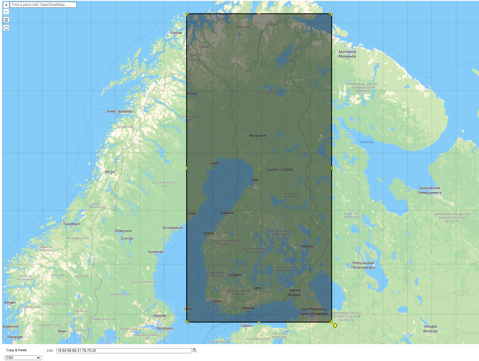
fin_bbox = 19.84, 59.68, 31.78, 70.25

Get data POIS

Fetch all POIS from our bounding box that covers Finland.

%%time

table = overturemaps.record_batch_reader("place", fin_bbox).read_all()

# Temporarily required as of Lonboard 0.8 to avoid a Lonboard bug
# table = table.combine_chunks()

CPU times: user 1.38 s, sys: 478 ms, total: 1.86 s
Wall time: 7.89 s

To Finland border

To get the data delimited to the Finland’s border we will use the Country Admin layer. Let’s download it into our working space first. We need to do this delimitation using Clip from Geopandas

We use this dataset due to quality accuracy.

!wget -N https://a3s.fi/swift/v1/AUTH_a6b8530017f34af9861fcf45a738ad3f/L2-CellTowers/L2-CountryAdmin-data.gpkg

--2024-07-08 16:32:18--  https://a3s.fi/swift/v1/AUTH_a6b8530017f34af9861fcf45a738ad3f/L2-CellTowers/L2-CountryAdmin-data.gpkg
Resolving a3s.fi (a3s.fi)... 86.50.254.18, 86.50.254.19
Connecting to a3s.fi (a3s.fi)|86.50.254.18|:443... connected.
HTTP request sent, awaiting response... 304 Not Modified
File ‘L2-CountryAdmin-data.gpkg’ not modified on server. Omitting download.

# read country layer
world_admin = gpd.read_file('L2-CountryAdmin-data.gpkg')

# clean and get needed columns
world_admin = world_admin.dropna()

world_gdf = world_admin[['name', 'continent', 'geometry']]

world_gdf.head(3)

	name	continent	geometry
0	Uganda	Africa	MULTIPOLYGON (((33.92110 -1.00194, 33.92027 -1...
1	Uzbekistan	Asia	MULTIPOLYGON (((70.97081 42.25467, 70.98054 42...
2	Ireland	Europe	MULTIPOLYGON (((-9.97014 54.02083, -9.93833 53...

# get Finland border
fin = world_gdf.loc[world_gdf['name']=='Finland']

ax = fin.plot();

ax.axis('off');

Let’s transform our arrow table into a geodataframe to operate the Clip

# to GeoDataFrame
geodata = gpd.GeoDataFrame(table.to_pandas(), 
                           geometry=gpd.GeoSeries.from_wkb(table['geometry'])
                          )

# Clip data to Finland
fin_pois = gpd.clip(geodata, fin)

fin_pois.head(3) 

	id	geometry	bbox	version	update_time	sources	names	categories	confidence	websites	socials	emails	phones	brand	addresses
80379	08f1126d13813811035492970601cdd4	POINT (25.02573 60.15663)	{'xmin': 25.025728225708008, 'xmax': 25.025732...	0	2024-05-10T00:00:00.000Z	[{'property': '', 'dataset': 'meta', 'record_i...	{'primary': 'Koivusaari', 'common': None, 'rul...	{'main': 'active_life', 'alternate': ['island']}	0.545360	None	[https://www.facebook.com/407047872667629]	None	None	None	[{'freeform': None, 'locality': 'Helsinki', 'p...
80394	08f1126d13b98c750373f6c5e88f8cfc	POINT (25.03381 60.16034)	{'xmin': 25.033811569213867, 'xmax': 25.033815...	0	2024-05-10T00:00:00.000Z	[{'property': '', 'dataset': 'meta', 'record_i...	{'primary': 'Tahvonlahdenniemi', 'common': Non...	{'main': 'attractions_and_activities', 'altern...	0.667112	None	[https://www.facebook.com/268426200024634]	None	None	None	[{'freeform': None, 'locality': None, 'postcod...
80396	08f1126d13710ca603d51db4e2126d09	POINT (25.04591 60.15272)	{'xmin': 25.045907974243164, 'xmax': 25.045911...	0	2024-05-10T00:00:00.000Z	[{'property': '', 'dataset': 'meta', 'record_i...	{'primary': 'Santahaminan ala-asteen koulu', '...	{'main': 'elementary_school', 'alternate': None}	0.917202	[https://www.hel.fi/peruskoulut/fi/koulut/sant...	[https://www.facebook.com/318142011597385]	None	[+358931089709]	None	[{'freeform': 'Santahaminantie 5', 'locality':...

len(fin_pois)

181531

# let's check how much memory is it using
memory_fin = fin_pois.memory_usage(index=True).sum()

print(f'Total memory used for GeoDataFrame: {memory_fin/1000000000} GB')

Total memory used for GeoDataFrame: 0.022509844 GB

# to Geoparquet
fin_pois.to_parquet('output/pois_finland.parquet', index=False)

Map from GeoDataFrame

Previously, we used the arrow table to visualization in lonboard. Now, we are going to test it using the converted GeoDataFrame.

YlGnBu_9.mpl_colormap

YlGnBu

under

bad

over

# let's apply the color palette

confidence_array = fin_pois['confidence'].to_numpy()

colors = apply_continuous_cmap(confidence_array, YlGnBu_9)

# ---- Create a Layer

layer = ScatterplotLayer.from_geopandas(
                                    # --- Select only a few attribute columns from the table
                
                                    fin_pois[["id", "categories", "geometry", "confidence"]],
                                    get_radius = np.array([500*value for value in fin_pois['confidence'].to_numpy()]),
                                    get_fill_color=colors,
                                )

view_state = {
    "longitude": 26.814052,
    "latitude": 62.399194,
    "zoom": 6,
    "pitch": 40,
    "bearing": 4,
}
m = Map(layer, view_state=view_state)

# set a name for html
html_file = 'finland_pois_border.html'

#path
html_path = os.path.join('output', html_file)

m.to_html(html_path)

# IFrame(src=html_path, width=1600 , height=700)

POIS Worldwide (Global)

Grid strategy

We are going to create a Grid that covers globally the fetching process. We will use our World Admin layer and define a grid size in degrees. Then, the strategy is to create a process that fetches POI data per Grid and stores it in the local disk. This process is the one we will parallelize per each Grid.

We use degrees to avoid projection issues. By using degrees we can divide the globe in exact numbers.

Check the next function

def create_grid(study_area, grid_size_m):
    '''
    Give back a Geodataframe with specific grid size based on study area
        study_area: geodaframe. default point geometry. crs not geographic
        grid_size_m: size of grid side in meters

        return: Geodataframe of polygons. Grid
    '''
    from shapely.geometry import Polygon
    
    print(f'CRS of study area: {study_area.crs.name}')
    
    # get bounds of province
    # xmin, ymin, xmax, ymax = study_area.buffer(100).total_bounds
    xmin, ymin, xmax, ymax = -180, -90, 180, 90

    # grid size
    length = grid_size_m
    wide = grid_size_m

    cols = list(np.arange(xmin, xmax + wide, wide))
    rows = list(np.arange(ymin, ymax + length, length))

    polygons = []
    for x in cols[:-1]:
        for y in rows[:-1]:
            polygons.append(Polygon([(x,y), (x+wide, y), (x+wide, y+length), (x, y+length)]))
    
    # grid = gpd.GeoDataFrame({'geometry':polygons}, crs = study_area.crs)
    grid = gpd.GeoDataFrame({'geometry':polygons}, crs = 4326)

    # ----- Remove empty grids

    index_true = []
    
    for row in grid.itertuples():

        # check if contains
        contains = study_area.intersects(row.geometry)
  
        if True in contains.unique():

            # catch index of grid that contains study area
            index_true.append(row.Index)

    # subset only valid grids
    grid_valid = grid.loc[grid.index.isin(index_true)]

    # reset index
    grid_valid = grid_valid.reset_index(drop=True)
    
    print(f'Total grids: {len(grid_valid)}')
    
    return grid_valid

Global limits covered

We will get a Geographic grid within the limits of the global boundaries.

We will start defining all Continents and Islands in the globe. We use the given country admin layer with high resolution that contains islands and we add the Antarctic from Natural Earth low resolution.

# using Natural Earth to add Antarctica
gdf = gpd.read_file(gpd.datasets.get_path('naturalearth_lowres'))

Antarctica = gdf.loc[gdf.continent=='Antarctica'][['name', 'geometry']];

# merge
world_gdf_globe = pd.concat([world_gdf[['name', 'geometry']], Antarctica])

print(f'Crs: {world_gdf_globe.crs.name}')

ax = world_gdf_globe.plot(figsize=(10,6))

ax.axis('off');

Crs: WGS 84

world_gdf_globe.crs.name

'WGS 84'

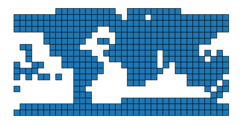
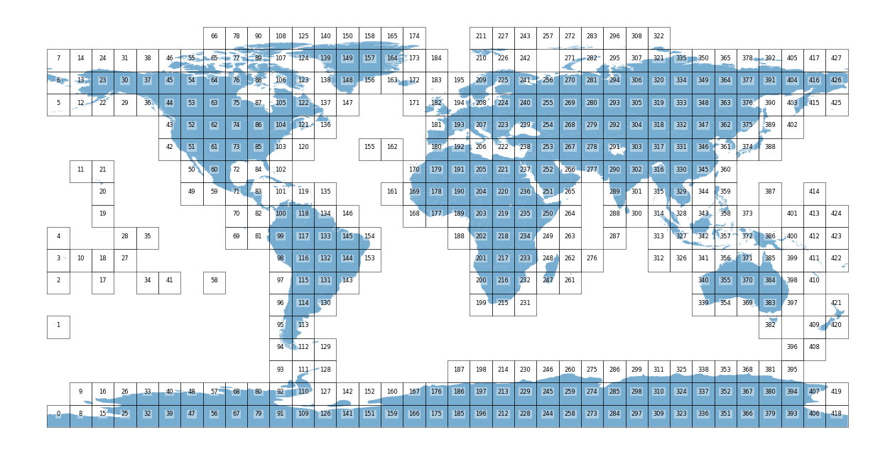
Grid creation and visualization

Let’s use our function create_grid. It will give back a WGS84 grid layer that is overlapped in the administrative boundaries defined above.

# create a global grid
grid_globe = create_grid(world_gdf_globe, 10)

CRS of study area: WGS 84
Total grids: 428

print(f'Total Cells: {len(grid_globe)}')

ax = grid_globe.plot(figsize=(10,6), edgecolor='black')

ax.axis('off');

Total Cells: 428

grid_globe.to_file('output/grid_global.gpkg')

fig, ax = plt.subplots(figsize=(16, 14))

# plot
world_gdf_globe.plot(ax=ax,
                       # color='darkblue',
                       # markersize= 3,
                       alpha = 0.6,
                      )

grid_globe.plot(ax=ax,
          facecolor="none", 
          edgecolor="black",
          linewidth=0.6,
          alpha=0.6
         )

# ------- lables
grid_globe['coords'] = grid_globe['geometry'].apply(lambda x: x.representative_point().coords[:][0])
grid_globe['index'] = grid_globe.index

for idx, row in grid_globe.iterrows():
    
    ax.text(row.coords[0], 
            row.coords[1], 
            s=row['index'], 
            horizontalalignment='center', 
            # color='red',
            fontsize=6,
            bbox={'facecolor': 'white', 'alpha':0.4, 'pad': 1, 'edgecolor':'none'})


plt.axis('off');

# a frame for names
names = gpd.GeoDataFrame({'name':[f'n{num}' for num in grid_globe.index], 
                          'geometry':grid_globe.geometry.centroid})

%%time

# view state pydeck
view_state = pydeck.ViewState(latitude=40, longitude=0, zoom=0)

# set height and width variables
view = pydeck.View(type="_GlobeView", controller=True)#, width=800, height=800)

layers = [
    pydeck.Layer(
                "GeoJsonLayer",
                id="world-admin",
                data=world_gdf_globe,
                stroked=False,
                filled=True,           
				get_fill_color=[8, 173, 225], #, [230, 230, 230], # grey
                # get_line_color=[8, 173, 225],
                line_width_min_pixels=0.6
                ),
    pydeck.Layer(
                "GeoJsonLayer",
                id="world-grid",
                data=grid_globe,
                stroked=True,
                filled=False,           
				# get_fill_color=[230, 230, 230],
                get_line_color=[75, 132, 216], #[216, 57, 57],
                line_width_min_pixels=1
                ),
    pydeck.Layer(
                "TextLayer",
                data=names,
                get_position="geometry.coordinates",
                get_size=12,
                get_color=[75, 132, 216], #[216, 57, 57],
                get_text="name",
                ),
          ]

deck = pydeck.Deck(
                views=[view],
                initial_view_state=view_state,
                layers=layers,
                map_provider=None,
                # Note that this must be set for the globe to be opaque
                parameters={"cull": True},
            )

# deck.to_html("output/map.html")

CPU times: user 450 ms, sys: 20.4 ms, total: 470 ms
Wall time: 469 ms

deck

Fetch POI data - Parallelization

As a good practice, we will add an index like001, 002, 003 etc that will keep the downloaded files sorted. The function has a universal rule that will keep the index fixed even if you make a smaller grid with four digits number.

# create index that sort filepaths
max = len(str(grid_globe.index.max()))

# wild card based on length
wild_card = '0'*max

# add to index col
grid_globe['index_path'] = [(wild_card+str(index))[-max:] for index in grid_globe.index]

def fetch_grid_data(grid, grid_index, grid_path, tag_name, output_folder):
    '''
    Fetch and store Overture Maps data using a Grid and Grid index.
        grid: GDF, in wgs84
        grid_index: int
        tag_name: one from "building" or "place"
        output_folder: output folder path
    '''


    # ----------- path
    
    # output name    
    output_name = f'Grid_{grid_path}_{tag_name}.parquet'

    output_path = os.path.join(output_folder, output_name)

    if not os.path.exists(output_path):
        
        # get the geom from grid using grid_index
        grid_geom = grid.at[grid_index, 'geometry']
    
        # get arrow table
        table = overturemaps.record_batch_reader(tag_name, grid_geom.bounds).read_all()
    
        # to GDF
        geodata = gpd.GeoDataFrame(table.to_pandas(), 
                                   geometry=gpd.GeoSeries.from_wkb(table['geometry'])
                                  )[['id', 'geometry', 'names', 'categories', 'confidence']]

        # add coordinates
        geodata['longitude'] = [geom.x for geom in geodata.geometry]
        geodata['latitude'] = [geom.y for geom in geodata.geometry]
                
        # --- Memory
        # memory = round(geodata.memory_usage(deep=True).sum()/1000000000, 1)
    
        # ----- Save
    
        # output path
        if not os.path.exists(output_folder):
            
            os.makedirs(output_folder)
    
        
        # to Geoparquet
        geodata.to_parquet(output_path, index=False)
    
        print(f'Saved: {output_name}')
        
        # remove from local memory
        table = None
        geodata = None
    
        
        gc.collect()
        
        
        # return (grid_index, round(memory, 2))

Dask delayed functions

As we coded our function to download the dataset per Grid, we are going to create a delayed function from Dask. These functions will run in parallel using the capabilities of the supercomputer distributing the capacity in every process. The advantage of using Dask delayed is that it keeps memory usage efficient. On the other hand, libraries like Multiprocess accumulate memory and break the session.

Keep in mind that we will download the data in scratch disk.

# parameters like: fetch_grid_data(grid, grid_index, grid_path, tag_name, output_folder)

# define scratch folder
scratch_folder = '/scratch/project_2009245/Overture-Global-POI'


# ----- get all object to process
all_delayed = []

# ------ loop in parameters

for grid_index, grid_path in zip(grid_globe.index, grid_globe.index_path):

    # create a delayed object
    delayed_object = dask.delayed(fetch_grid_data)(grid_globe, grid_index, grid_path, 'place', scratch_folder)

    all_delayed.append(delayed_object)

# delayed_object.visualize()

s = time.time()

# --- run all delayed functions

dask.compute(all_delayed)

# -------- 
time_parallel = time.time() - s

Saved: Grid_392_place.parquet
Saved: Grid_112_place.parquet
Saved: Grid_156_place.parquet
Saved: Grid_212_place.parquet
Saved: Grid_123_place.parquet
Saved: Grid_168_place.parquet
Saved: Grid_292_place.parquet
Saved: Grid_217_place.parquet
Saved: Grid_409_place.parquet
Saved: Grid_416_place.parquet
Saved: Grid_310_place.parquet
Saved: Grid_415_place.parquet
Saved: Grid_027_place.parquet
Saved: Grid_036_place.parquet
Saved: Grid_179_place.parquet
Saved: Grid_330_place.parquet
Saved: Grid_260_place.parquet
Saved: Grid_326_place.parquet
Saved: Grid_065_place.parquet
Saved: Grid_286_place.parquet
Saved: Grid_343_place.parquet
Saved: Grid_171_place.parquet
Saved: Grid_137_place.parquet
Saved: Grid_250_place.parquet
Saved: Grid_060_place.parquet
Saved: Grid_077_place.parquet
Saved: Grid_371_place.parquet
Saved: Grid_049_place.parquet
Saved: Grid_094_place.parquet
Saved: Grid_314_place.parquet
Saved: Grid_018_place.parquet
Saved: Grid_240_place.parquet
Saved: Grid_214_place.parquet
Saved: Grid_361_place.parquet
Saved: Grid_056_place.parquet
Saved: Grid_139_place.parquet
Saved: Grid_045_place.parquet
Saved: Grid_395_place.parquet
Saved: Grid_349_place.parquet
Saved: Grid_379_place.parquet
Saved: Grid_124_place.parquet
Saved: Grid_284_place.parquet
Saved: Grid_070_place.parquet
Saved: Grid_401_place.parquet
Saved: Grid_083_place.parquet
Saved: Grid_043_place.parquet
Saved: Grid_158_place.parquet
Saved: Grid_398_place.parquet
Saved: Grid_173_place.parquet
Saved: Grid_174_place.parquet
Saved: Grid_162_place.parquet
Saved: Grid_113_place.parquet
Saved: Grid_272_place.parquet
Saved: Grid_193_place.parquet
Saved: Grid_068_place.parquet
Saved: Grid_311_place.parquet
Saved: Grid_223_place.parquet
Saved: Grid_354_place.parquet
Saved: Grid_182_place.parquet
Saved: Grid_023_place.parquet
Saved: Grid_072_place.parquet
Saved: Grid_129_place.parquet
Saved: Grid_133_place.parquet
Saved: Grid_421_place.parquet
Saved: Grid_302_place.parquet
Saved: Grid_047_place.parquet
Saved: Grid_050_place.parquet
Saved: Grid_278_place.parquet
Saved: Grid_350_place.parquet
Saved: Grid_107_place.parquet
Saved: Grid_269_place.parquet
Saved: Grid_218_place.parquet
Saved: Grid_367_place.parquet
Saved: Grid_232_place.parquet
Saved: Grid_271_place.parquet
Saved: Grid_423_place.parquet
Saved: Grid_394_place.parquet
Saved: Grid_144_place.parquet
Saved: Grid_342_place.parquet
Saved: Grid_025_place.parquet
Saved: Grid_006_place.parquet
Saved: Grid_095_place.parquet
Saved: Grid_234_place.parquet
Saved: Grid_238_place.parquet
Saved: Grid_101_place.parquet
Saved: Grid_362_place.parquet
Saved: Grid_389_place.parquet
Saved: Grid_213_place.parquet
Saved: Grid_252_place.parquet
Saved: Grid_109_place.parquet
Saved: Grid_190_place.parquet
Saved: Grid_317_place.parquet
Saved: Grid_004_place.parquet
Saved: Grid_067_place.parquet
Saved: Grid_216_place.parquet
Saved: Grid_093_place.parquet
Saved: Grid_257_place.parquet
Saved: Grid_258_place.parquet
Saved: Grid_130_place.parquet
Saved: Grid_412_place.parquet
Saved: Grid_320_place.parquet
Saved: Grid_399_place.parquet
Saved: Grid_086_place.parquet
Saved: Grid_344_place.parquet
Saved: Grid_325_place.parquet
Saved: Grid_069_place.parquet
Saved: Grid_042_place.parquet
Saved: Grid_051_place.parquet
Saved: Grid_110_place.parquet
Saved: Grid_244_place.parquet
Saved: Grid_370_place.parquet
Saved: Grid_262_place.parquet
Saved: Grid_267_place.parquet
Saved: Grid_136_place.parquet
Saved: Grid_270_place.parquet
Saved: Grid_202_place.parquet
Saved: Grid_169_place.parquet
Saved: Grid_256_place.parquet
Saved: Grid_224_place.parquet
Saved: Grid_167_place.parquet
Saved: Grid_038_place.parquet
Saved: Grid_274_place.parquet
Saved: Grid_340_place.parquet
Saved: Grid_150_place.parquet
Saved: Grid_418_place.parquet
Saved: Grid_427_place.parquet
Saved: Grid_241_place.parquet
Saved: Grid_146_place.parquet
Saved: Grid_316_place.parquet
Saved: Grid_291_place.parquet
Saved: Grid_380_place.parquet
Saved: Grid_128_place.parquet
Saved: Grid_181_place.parquet
Saved: Grid_014_place.parquet
Saved: Grid_085_place.parquet
Saved: Grid_406_place.parquet
Saved: Grid_368_place.parquet
Saved: Grid_001_place.parquet
Saved: Grid_305_place.parquet
Saved: Grid_300_place.parquet
Saved: Grid_053_place.parquet
Saved: Grid_226_place.parquet
Saved: Grid_096_place.parquet
Saved: Grid_189_place.parquet
Saved: Grid_141_place.parquet
Saved: Grid_029_place.parquet
Saved: Grid_347_place.parquet
Saved: Grid_422_place.parquet
Saved: Grid_374_place.parquet
Saved: Grid_312_place.parquet
Saved: Grid_108_place.parquet
Saved: Grid_125_place.parquet
Saved: Grid_048_place.parquet
Saved: Grid_082_place.parquet
Saved: Grid_287_place.parquet
Saved: Grid_131_place.parquet
Saved: Grid_297_place.parquet
Saved: Grid_206_place.parquet
Saved: Grid_175_place.parquet
Saved: Grid_134_place.parquet
Saved: Grid_309_place.parquet
Saved: Grid_259_place.parquet
Saved: Grid_387_place.parquet
Saved: Grid_211_place.parquet
Saved: Grid_062_place.parquet
Saved: Grid_419_place.parquet
Saved: Grid_012_place.parquet
Saved: Grid_282_place.parquet
Saved: Grid_247_place.parquet
Saved: Grid_403_place.parquet
Saved: Grid_383_place.parquet
Saved: Grid_163_place.parquet
Saved: Grid_028_place.parquet
Saved: Grid_026_place.parquet
Saved: Grid_222_place.parquet
Saved: Grid_076_place.parquet
Saved: Grid_000_place.parquet
Saved: Grid_002_place.parquet
Saved: Grid_253_place.parquet
Saved: Grid_061_place.parquet
Saved: Grid_319_place.parquet
Saved: Grid_192_place.parquet
Saved: Grid_248_place.parquet
Saved: Grid_408_place.parquet
Saved: Grid_357_place.parquet
Saved: Grid_201_place.parquet
Saved: Grid_209_place.parquet
Saved: Grid_348_place.parquet
Saved: Grid_390_place.parquet
Saved: Grid_091_place.parquet
Saved: Grid_372_place.parquet
Saved: Grid_290_place.parquet
Saved: Grid_254_place.parquet
Saved: Grid_044_place.parquet
Saved: Grid_337_place.parquet
Saved: Grid_425_place.parquet
Saved: Grid_057_place.parquet
Saved: Grid_003_place.parquet
Saved: Grid_322_place.parquet
Saved: Grid_197_place.parquet
Saved: Grid_426_place.parquet
Saved: Grid_420_place.parquet
Saved: Grid_276_place.parquet
Saved: Grid_264_place.parquet
Saved: Grid_007_place.parquet
Saved: Grid_281_place.parquet
Saved: Grid_199_place.parquet
Saved: Grid_369_place.parquet
Saved: Grid_041_place.parquet
Saved: Grid_249_place.parquet
Saved: Grid_114_place.parquet
Saved: Grid_066_place.parquet
Saved: Grid_170_place.parquet
Saved: Grid_283_place.parquet
Saved: Grid_386_place.parquet
Saved: Grid_078_place.parquet
Saved: Grid_166_place.parquet
Saved: Grid_268_place.parquet
Saved: Grid_382_place.parquet
Saved: Grid_159_place.parquet
Saved: Grid_385_place.parquet
Saved: Grid_352_place.parquet
Saved: Grid_324_place.parquet
Saved: Grid_185_place.parquet
Saved: Grid_016_place.parquet
Saved: Grid_118_place.parquet
Saved: Grid_098_place.parquet
Saved: Grid_138_place.parquet
Saved: Grid_215_place.parquet
Saved: Grid_353_place.parquet
Saved: Grid_099_place.parquetSaved: Grid_328_place.parquet

Saved: Grid_157_place.parquet
Saved: Grid_022_place.parquet
Saved: Grid_058_place.parquet
Saved: Grid_132_place.parquet
Saved: Grid_207_place.parquet
Saved: Grid_358_place.parquet
Saved: Grid_198_place.parquet
Saved: Grid_115_place.parquet
Saved: Grid_188_place.parquet
Saved: Grid_031_place.parquet
Saved: Grid_116_place.parquet
Saved: Grid_073_place.parquet
Saved: Grid_102_place.parquet
Saved: Grid_227_place.parquet
Saved: Grid_104_place.parquet
Saved: Grid_261_place.parquet
Saved: Grid_246_place.parquet
Saved: Grid_273_place.parquet
Saved: Grid_295_place.parquet
Saved: Grid_225_place.parquet
Saved: Grid_019_place.parquet
Saved: Grid_375_place.parquet
Saved: Grid_299_place.parquet
Saved: Grid_323_place.parquet
Saved: Grid_365_place.parquet
Saved: Grid_194_place.parquet
Saved: Grid_373_place.parquet
Saved: Grid_251_place.parquet
Saved: Grid_255_place.parquet
Saved: Grid_304_place.parquet
Saved: Grid_275_place.parquet
Saved: Grid_090_place.parquet
Saved: Grid_208_place.parquet
Saved: Grid_411_place.parquet
Saved: Grid_243_place.parquet
Saved: Grid_391_place.parquet
Saved: Grid_237_place.parquet
Saved: Grid_039_place.parquet
Saved: Grid_219_place.parquet
Saved: Grid_196_place.parquet
Saved: Grid_079_place.parquet
Saved: Grid_200_place.parquet
Saved: Grid_413_place.parquet
Saved: Grid_266_place.parquet
Saved: Grid_221_place.parquet
Saved: Grid_381_place.parquet
Saved: Grid_318_place.parquet
Saved: Grid_121_place.parquet
Saved: Grid_402_place.parquet
Saved: Grid_122_place.parquet
Saved: Grid_030_place.parquet
Saved: Grid_154_place.parquet
Saved: Grid_164_place.parquet
Saved: Grid_005_place.parquet
Saved: Grid_351_place.parquet
Saved: Grid_204_place.parquet
Saved: Grid_081_place.parquet
Saved: Grid_400_place.parquet
Saved: Grid_009_place.parquet
Saved: Grid_105_place.parquet
Saved: Grid_388_place.parquet
Saved: Grid_151_place.parquet
Saved: Grid_054_place.parquet
Saved: Grid_008_place.parquet
Saved: Grid_308_place.parquet
Saved: Grid_074_place.parquet
Saved: Grid_313_place.parquet
Saved: Grid_220_place.parquet
Saved: Grid_210_place.parquet
Saved: Grid_377_place.parquet
Saved: Grid_135_place.parquet
Saved: Grid_329_place.parquet
Saved: Grid_417_place.parquet
Saved: Grid_024_place.parquet
Saved: Grid_294_place.parquet
Saved: Grid_119_place.parquet
Saved: Grid_178_place.parquet
Saved: Grid_303_place.parquet
Saved: Grid_180_place.parquet
Saved: Grid_424_place.parquet
Saved: Grid_020_place.parquet
Saved: Grid_327_place.parquet
Saved: Grid_331_place.parquet
Saved: Grid_097_place.parquet
Saved: Grid_153_place.parquet
Saved: Grid_089_place.parquet
Saved: Grid_356_place.parquet
Saved: Grid_172_place.parquet
Saved: Grid_120_place.parquet
Saved: Grid_183_place.parquet
Saved: Grid_184_place.parquet
Saved: Grid_032_place.parquet
Saved: Grid_228_place.parquet
Saved: Grid_306_place.parquet
Saved: Grid_080_place.parquet
Saved: Grid_296_place.parquet
Saved: Grid_298_place.parquet
Saved: Grid_126_place.parquet
Saved: Grid_176_place.parquet
Saved: Grid_010_place.parquet
Saved: Grid_233_place.parquet
Saved: Grid_037_place.parquet
Saved: Grid_378_place.parquet
Saved: Grid_015_place.parquet
Saved: Grid_293_place.parquet
Saved: Grid_203_place.parquet
Saved: Grid_064_place.parquet
Saved: Grid_363_place.parquet
Saved: Grid_071_place.parquet
Saved: Grid_152_place.parquet
Saved: Grid_011_place.parquet
Saved: Grid_339_place.parquet
Saved: Grid_245_place.parquet
Saved: Grid_288_place.parquet
Saved: Grid_231_place.parquet
Saved: Grid_161_place.parquet
Saved: Grid_052_place.parquet
Saved: Grid_147_place.parquet
Saved: Grid_088_place.parquet
Saved: Grid_397_place.parquet
Saved: Grid_103_place.parquet
Saved: Grid_279_place.parquet
Saved: Grid_239_place.parquet
Saved: Grid_195_place.parquet
Saved: Grid_321_place.parquet
Saved: Grid_396_place.parquet
Saved: Grid_332_place.parquet
Saved: Grid_017_place.parquetSaved: Grid_376_place.parquet

Saved: Grid_087_place.parquet
Saved: Grid_013_place.parquet
Saved: Grid_236_place.parquet
Saved: Grid_384_place.parquet
Saved: Grid_277_place.parquet
Saved: Grid_100_place.parquet
Saved: Grid_021_place.parquet
Saved: Grid_336_place.parquet
Saved: Grid_035_place.parquet
Saved: Grid_301_place.parquet
Saved: Grid_335_place.parquet
Saved: Grid_404_place.parquet
Saved: Grid_307_place.parquet
Saved: Grid_289_place.parquet
Saved: Grid_285_place.parquet
Saved: Grid_346_place.parquet
Saved: Grid_414_place.parquet
Saved: Grid_063_place.parquet
Saved: Grid_359_place.parquet
Saved: Grid_345_place.parquet
Saved: Grid_143_place.parquet

print(f'Total time in Parallel download: {time_parallel/60} mins') # 27 mins 

# ------ 45 mins 2 cores 60 - 80 Disk RES 31GB
# ------ 34 mins 4 cores 60 - 80 Disk RES 31GB
# ------ 25. mins 8 cores 60 - 80 Disk 34 GB

Total time in Parallel download: 25.22586595217387 mins

Memory profile

If you want to understand the capacity that you require for your supercomputer session (Jupyter) you can open a dashboard in your terminal with:

$ top -u $USER

Then, you can check in RES the max memory that your memory used. In this case this process gave 32GB and our capacity was 60GB. So, we can still ask for less resources in our supercomputer session.

Analyze Global POIS

The PyArrow Python library can be fascinating while using the GeoParquet format. You simply need to add the parquet files with indexation and a common name in a folder and then simply direct the folder. In our case, we stored our files like Grid_000_place.parquet, Grid_001_place.parquet, Grid_002_place.parquet, etc in the folder Overture-Global-POI. So, we simply need to point the folder to read all files at the same time.

# define scratch folder
scratch_folder = '/scratch/project_2009245/Overture-Global-POI'

# ------------ read all data

global_pois = pq.read_table(scratch_folder)

len(global_pois)

52611458

type(global_pois)

pyarrow.lib.Table

global_pois.column_names

['id',
 'geometry',
 'names',
 'categories',
 'confidence',
 'longitude',
 'latitude']

global_pois.select(['confidence']).to_pandas().confidence.mean()

0.6620629039050556

Operations in arrow table

You can learn about operations and transformation in the arrow format for arrays and tables in the Arrow Cookbook. Arrow contains a function called compute similar to Dask that you use when you want to run the transformation.

Let’s check some examples. The purpose of this analysis is to answer the question.

What is the most frequent main category at the global level?

import pyarrow.compute as compute
import pyarrow as arrow

type(global_pois)

pyarrow.lib.Table

Global confidence mean

A numerical operation in the global dataset using arrow.array

# define column
column_array = arrow.array(global_pois["confidence"])

# get compute mean
global_confidence_mean = compute.mean(column_array)

print(global_confidence_mean)

0.6620629039050578

Add a new column in PyArrow

The categories of use of every POI is stored in the categories column as a dicitionary. To get the main category we need to simply call the key and we will have back the main category.

We will create a function main_group that will give back the main category, in a new column. We will apply this function on the fly by using append_column

def main_group(dict_str):
    '''
    Gives back the main group of POIS
    '''
    # add condition

    if 'main' in dict_str.keys():
        
        # get main group
        main = dict_str['main']

        return main   

    else:

        main = None

        return main    

%%time

# -- it might take some time

# add a column as an arrow array
new_column = arrow.array(global_pois['categories'])

CPU times: user 4min 42s, sys: 1.55 s, total: 4min 44s
Wall time: 4min 43s

%%time

# add arrow column -  and apply the function right away

global_pois = global_pois.append_column(
                                        'main_group',
                                        arrow.array([main_group(categories) for categories in new_column])                                        
                                        )

CPU times: user 2min 32s, sys: 1.09 s, total: 2min 33s
Wall time: 2min 34s

Count values

The function value_counts gives back a dictionary with the occurrence of every main category. We will separate it in a DataFrame to plot it

%%time

# count the occurrence of main groups
occurrence = compute.value_counts(arrow.array(global_pois['main_group']))

CPU times: user 46.2 s, sys: 852 ms, total: 47.1 s
Wall time: 46.9 s

type(occurrence)

pyarrow.lib.StructArray

Summary table and plot

Summarizing in a table.

# get arrays of summary
group_array = occurrence.field('values')
count_array = occurrence.field('counts')

# create a dataframe with summarized groups
group_df = pd.DataFrame({'main':group_array, 'count':count_array}).sort_values('count', ascending=False).reset_index(drop=True)

group_df.isna().sum()

main     1
count    0
dtype: int64

# filter non values
group_df.dropna(inplace=True)

group_df.isna().sum()

main     0
count    0
dtype: int64

# define a top 20

group_occ = group_df[:20]

group_occ

	main	count
1	beauty_salon	1821129
2	hotel	1154008
3	professional_services	982381
4	landmark_and_historical_building	952504
5	restaurant	898470
6	shopping	845410
7	school	782504
8	hospital	732171
9	church_cathedral	712911
10	cafe	708970
11	community_services_non_profits	682931
12	bar	646338
13	automotive_repair	633625
14	park	525446
15	real_estate	513000
16	clothing_store	506267
17	coffee_shop	503422
18	dentist	461274
19	gym	455613
20	grocery_store	410280

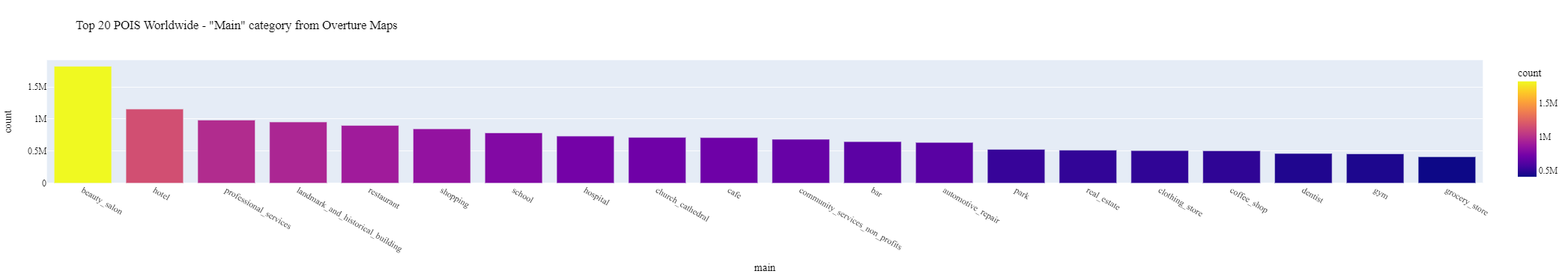
# plotly

fig = px.bar(group_occ, 
             height=600,
             x='main', 
             y='count',
             color='count',
             hover_data=['main', 'count'],
             title='Top 20 POIS Worldwide - "Main" category from Overture Maps'
            )

# update font
fig.update_layout(
    font=dict(size=14),
    font_family="Times New Roman",
    font_color="black",
    title_font_family="Times New Roman",
)

fig.show()

Global visualization of POIS

We will continue visualizing the data by filtering the main_group column. Also, checking how to filter a table with Arrow using filter

global_pois.column_names

['id',
 'geometry',
 'names',
 'categories',
 'confidence',
 'longitude',
 'latitude',
 'main_group']

Filter table by expression

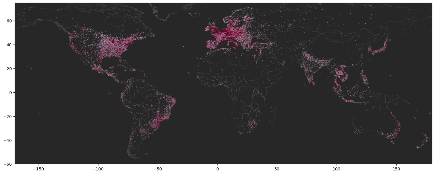
Let’s get from the global data only the beauty salon main category

len(global_pois)

52611458

# get a new arrow table
main_global_pois = global_pois.filter(compute.field('main_group')=='beauty_salon')

len(main_global_pois)

1821129

main_global_pois.column_names

['id',
 'geometry',
 'names',
 'categories',
 'confidence',
 'longitude',
 'latitude',
 'main_group']

Visualize

We will check the data using DataShader as it is an efficient visualization library for point data. If you want to use different colors you can check the guide in the Colorcet Guide.

Let’s start creating a GeoDataFrame of our filtered data.

# --- define viz geodata

viz_geodata = gpd.GeoDataFrame(
                            main_global_pois.select(['main_group', 'longitude', 'latitude']).to_pandas(), 
                            geometry=gpd.GeoSeries.from_wkb(main_global_pois['geometry'])
                          )

%%time

# canvas object
canvas = ds.Canvas(plot_width=900, plot_height=500)

# variable columns aggregation like agg=ds.max("column-name") Polygon or ds.count_cat('cat') category
agg = canvas.points(viz_geodata, geometry='geometry', agg=ds.count())

# image shade with a distribution like ‘eq_hist’ [default], ‘cbrt’ (cube root), ‘log’ (logarithmic), and ‘linear’
# cmaps like fire, kb, kr, kg, bgyw, rainbow4

im = ds_function.shade(agg, cmap=cc.CET_D10, how='eq_hist')

ds_function.set_background(im, "#272727") # #0A0A0A

# save
export = partial(export_image, background = "#272727", export_path='output')
export(im, 'beauty_salon_pois_overture')

CPU times: user 1.61 s, sys: 8.88 ms, total: 1.62 s
Wall time: 1.6 s

Visualize H3 aggregation

If you want to make ‘’lighter’’ visualizations you can also aggregate the data into H3 Hexagons using the H3 Pandas Python library. The function that counts the occurrence into every hexagon is h3.geo_to_h3_aggregate().

# aggregate occurrence into every hexagon
global_h3_pois = viz_geodata.h3.geo_to_h3_aggregate(resolution=5,
                                                    operation='count',
                                                    lng_col='longitude',
                                                    lat_col='latitude'
                                                   )

# global_h3_pois_index.dropna(inplace=True)

global_h3_pois.head()

	main_group	geometry
h3_05
85012067fffffff	1	POLYGON ((24.65287 70.98998, 24.81422 71.04301...
850120abfffffff	1	POLYGON ((23.70738 70.67050, 23.86232 70.72389...
850120bbfffffff	13	POLYGON ((23.64504 70.54437, 23.79861 70.59766...
850122a3fffffff	3	POLYGON ((26.14638 70.85947, 26.31182 70.91115...
850122affffffff	1	POLYGON ((26.22929 70.98582, 26.39628 71.03757...

For now we will use a static visualization with Matplotlib. If you consider using a dynamic library like lonboard it might have difficulties to render.

ax = global_h3_pois.plot(figsize=(18,14), 
                        column='main_group', 
                        cmap='PuRd', 
                        scheme='quantiles',
                        zorder=1)

# add countries
world_gdf_globe.boundary.plot(ax=ax, 
                              zorder=0,
                             linewidth=0.1,
                              color='gray'
                             )

# plt.figure(facecolor='black')
ax.set_facecolor("#272727")

xlim = ([-170, 180])
ylim = ([-60, 75])

ax.set_xlim(xlim)
ax.set_ylim(ylim)

plt.savefig('output/global_pois_beauty_salon.png', dpi=300)

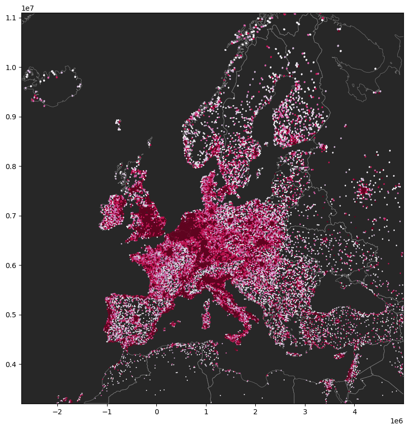
Let’s give a zoom in to understand better the H3 resolution you have used. You can also increase and have a more detailed map.

ax = global_h3_pois.to_crs(3857).plot(figsize=(10,10), 
                                        column='main_group', 
                                        cmap='PuRd', 
                                        scheme='quantiles',
                                        zorder=1)

# add countries
world_gdf_globe.to_crs(3857).boundary.plot(ax=ax, 
                                              zorder=0,
                                              linewidth=0.5,
                                              color='gray'
                                             )

# plt.figure(facecolor='black')
ax.set_facecolor("#272727")

# ----- Choose country to zoom

country_zoom = ['Iceland', 'Finland', 'Spain', 'Turkey']
country = world_gdf_globe.loc[world_gdf_globe['name'].isin(country_zoom)].to_crs(3857)

xlim = ([country.total_bounds[0],  country.total_bounds[2]])
ylim = ([country.total_bounds[1],  country.total_bounds[3]])

ax.set_xlim(xlim)
ax.set_ylim(ylim)

(3203347.2306077722, 11097617.58299868)