Using GIS libraries on Puhti#
In Puhti supercomputer there is an already installed environment for geospatial analysis called Geoconda. Geoconda is a customized Python environment for geospatial analysis. It contains a wide variety of packages for geospatial data processing, analysis, and visualization. The most common ones that will be used in the next tutorials are: geopandas, dask-geopandas, osmnx, datashader, and matplotlib.
This environment must be set up during the Jupyter session. The following steps will guide you through the process of loading the Geoconda environment in CSC’s Puhti supercomputer.
Geoconda was developed by CSC-IT Center for Science and Geoportti. You can find more information in the Geoconda documentation.
Follow the next steps in order to load Geoconda for the next tutorials.
Log in to Puhti#
The first step to start with High Performance Computing (HPC) is to log in in the CSC Puhti supercomputer.
CSC Puhti!
To log in to the web interface of Puhti supercomputer you need a CSC account or HAKA credentials. Be sure that you have been granted resources as explained in the previous section.
Set up a Jupyter Session#
The Puhti supercomputer has a user interface that allows you to access different applications like Visual Studio Code, Julia, MATLAB, MLflow, RStudio, TensorBoard, and the one we will use Jupyter.
To access the Jupyter Lab application you navigate to the User Interface menu in the Puhti dashboard or opening the Apps menu in the upper menu. If are logged in you can access to the dashboard using this link:
CSC Puhti dashboard!
To access Puhti dashboard you need to log in with a CSC account or HAKA credentials.
Simply, to start the JupyterLab click on the Jupyter button, like in Figure 1.
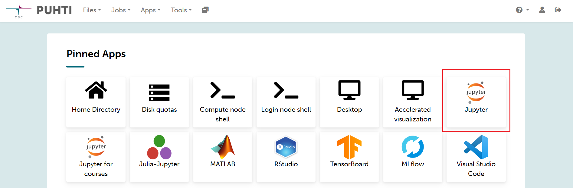
Figure 1. Puhti - Dashboard and Jupyter#
Then, you need to configure the needed resources for your Jupyter session. Be sure you have selected your own project like project_200xxxx. In this case, we are using partition interactive which has maximum 8 cores which is enough for our need. If you are willing to know more about the partitions find it in the Puhti Partitions Documentation.
For our parameters we will reserve 8 cores, 32 GB of processing memory, 60 GB of local disk, and 2 hours of availability. Your resources for now should look like Figure 2. Be sure that you are using your resources personally.
Note
If more people is sharing resources this configuration is not optimal and you must decrease resources.

Figure 2. Puhti - Jupyter configuration#
If you continue scrolling down you will find the Settings section. Under the Python parameter you should choose geoconda. Then in Module version you select the Geoconda version. We will work using the latest version (default). Finally, select your Working directory. It is recommended to use the disk scratch for working especially if you plan to write a large amount of results.
The Settings section might look like Figure 3.
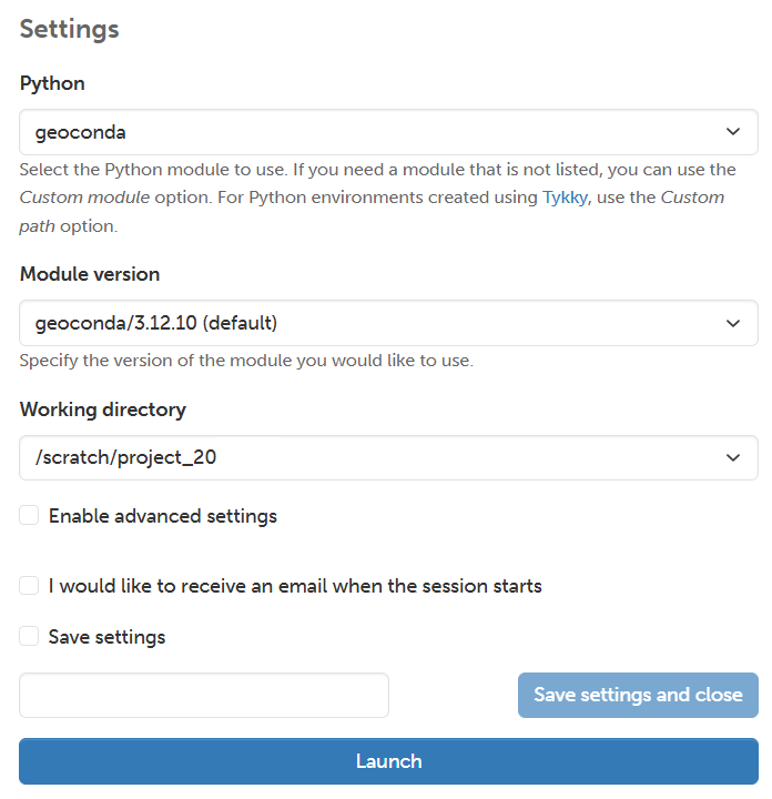
Figure 3. Puhti - Jupyter and Geoconda environment#
Finally, press the Launch button. You will see the session is launching untill it confirms it is Running. It will look like Figure 4.
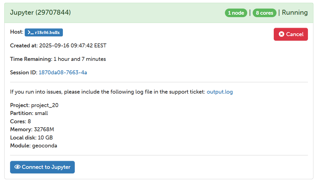
Figure 4. Puhti - Jupyter and Custom Python interpreter#
Then, press the button Connect to Jupyter and Jupyter Lab will open.
Clone the GeoHPC Repository#
In the Jupyter Lab interface, first create a new folder where you will clone the repository with the materials for the lessons. For this practice, we will call it GIT-HPC. You can create a new folder by using right-click in the Directory section and selecting New Folder. Then, navigate inside the folder GIT-HPC open a new terminal by clicking the Terminal icon in the Launcher menu like in Figure 5.
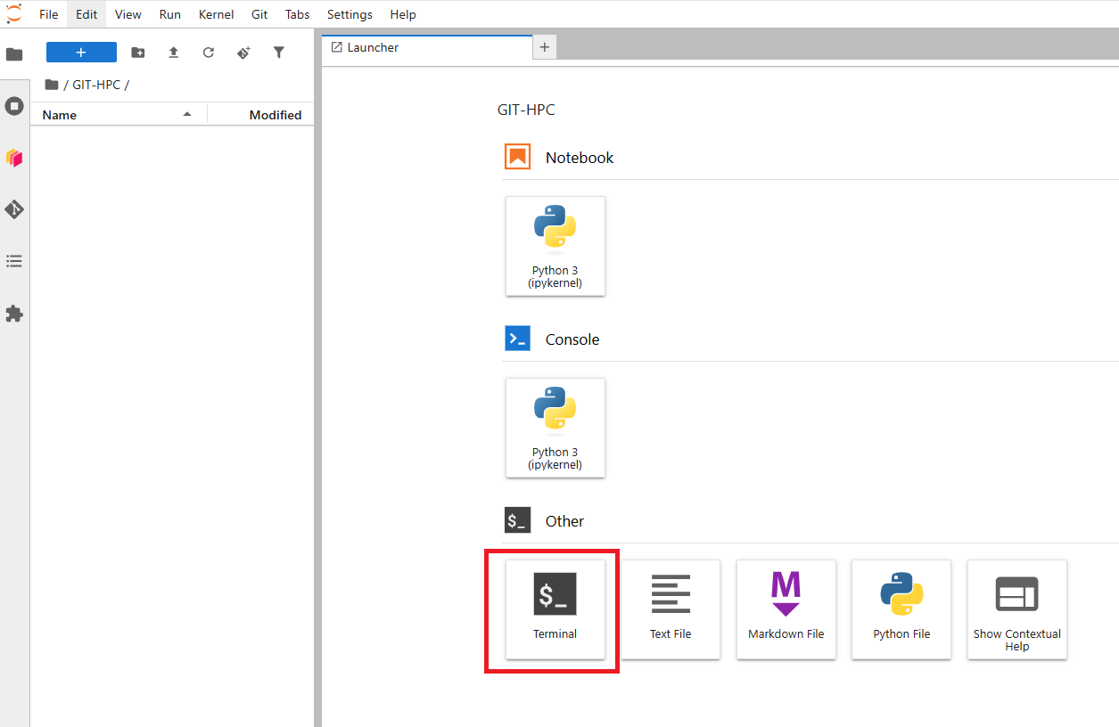
Figure 5. Puhti - Jupyter Lab and Terminal#
Once the terminal is open you can clone the GeoHPC repository using the following command:
git clone https://github.com/AaltoGIS/GeoHPC.git
Once you have cloned the GeoHPC repository you will find the Jupyter Notebook lessons under the folder:
/GIT-HPC/GeoHPC/source/lessons
The Jupyter Notebooks for every lessons are in every enumerated folder. For example, the notebook for lesson 1 in L1, and so on. The notebook name contains simply keywords of the lesson like Shortest Path.
Open the Jupyter Notebook of Lesson 1 from:
/GIT-HPC/GeoHPC/source/lessons/L1/01_ShortestPath-Parallelization.ipynb
If you have reached until here you are able to start the Lesson 1 using HPC resources and a customized environment container. Follow up the instruction in the Jupyter Notebook. You will be informed at the beginning of each lesson if you need to load Geoconda or a customized environment.
Happy coding!.