Lesson 1. Point aggregation

Aggregation of Cell Towers at country level worldwide

Introduction

In this Lesson, we are going to aggregate a global dataset of Cell Towers at country level. Commonly, the aggregation points-polygons or polygons-points is done using Spatial Join which is incorporated in the common Python library Geopandas for spatial analysis. Geopandas has improved considerably and the aggregation runs quite fast. But, as we are exploring parallelization, we will test the library Dask which is designed to use the computational resources in parallel. Also, there is an integration to Geopandas which is Dask-Geopandas that will be used to compare the time processing with and without parallelization.

This exercise is designed for teaching purposes of Spatial Data Science with High Performance Computing (HPC) at Aalto University. Thanks to the computational resources provided by CSC this exercise was tested in the Puhti supercomputer using Jupyter sessions.

Objective

To improve the processing time of a spatial join at a global level using Dask-Geopandas

Datasets

Cell Towers from OpenCellID

The database of Cell Towers was downloaded from OpenCellID and stored in Allas for your availability. The compressed file is ~1 GB and decompressed is ~5 GB. You will download it directly on your supercomputer.

Country admin level

The country border layer was downloaded from Natural Earth and stored in Allas for your availability. The Geopackage file is ~4 MB.

Output

The outputs of the spatial join are:

• (Polygon) Country borders with numbers of Cell Towers

• (Points) Cell Towers with attribute based con overlapping country

GIS env

This lessons uses Geoconda 🌎

HPC resources

CSC Puhti supercomputer:

• Partition: small

• CPU Cores: 8

• Memory (GB): 64

• Local Disk (GB): 10

Download dataset from Allas

The datasets for this practice are stored in Allas and can be downloaded to your local using the next commands. Simply, run the next cells.

!wget -N https://a3s.fi/L2-CellTowers/L2-CellTowers-data.csv.gz

--2025-09-23 09:47:54--  https://a3s.fi/L2-CellTowers/L2-CellTowers-data.csv.gz
Resolving a3s.fi (a3s.fi)... 86.50.254.18, 86.50.254.19
Connecting to a3s.fi (a3s.fi)|86.50.254.18|:443... connected.
HTTP request sent, awaiting response... 304 Not Modified
File ‘L2-CellTowers-data.csv.gz’ not modified on server. Omitting download.

!wget -N https://a3s.fi/L2-CellTowers/L2-CountryAdmin-data.gpkg

--2025-09-23 09:47:54--  https://a3s.fi/L2-CellTowers/L2-CountryAdmin-data.gpkg
Resolving a3s.fi (a3s.fi)... 86.50.254.19, 86.50.254.18
Connecting to a3s.fi (a3s.fi)|86.50.254.19|:443... connected.
HTTP request sent, awaiting response... 304 Not Modified
File ‘L2-CountryAdmin-data.gpkg’ not modified on server. Omitting download.

Decompress the Cell Tower data.

!gzip -d -f -k L2-CellTowers-data.csv.gz

Hands-on coding

Follow the instructions and run every cell in the supercomputer.

Importing Python libraries

Be sure that you have installed the dask_geopandas in your environment. Get familiar with this library reading a bit the Dask-Geopandas Documentation

import os

# -- for GIS
import pandas as pd
import geopandas as gpd
import dask_geopandas as geodask
import dask
import pyarrow
import numpy as np

# -- for Visualization
import matplotlib.pyplot as plt
import pydeck
import datashader as ds
import datashader.transfer_functions as ds_function
from datashader.utils import export_image
from functools import partial
import colorcet as cc

import time
import warnings
warnings.simplefilter("ignore")

# results folder
if not os.path.exists('output'):
    os.makedirs('output')

Read country layer

We will use the country’s administrative border for the Spatial Join. Beforehand, we do a test using a single country with the spatial operation within.

# read country layer
world_admin = gpd.read_file('L2-CountryAdmin-data.gpkg')

# clean and get needed columns
world_admin = world_admin.dropna()

world_gdf = world_admin[['iso3', 'name', 'continent', 'geometry']]

world_gdf.head()

	iso3	name	continent	geometry
0	UGA	Uganda	Africa	MULTIPOLYGON (((33.9211 -1.00194, 33.92027 -1....
1	UZB	Uzbekistan	Asia	MULTIPOLYGON (((70.97081 42.25467, 70.98054 42...
2	IRL	Ireland	Europe	MULTIPOLYGON (((-9.97014 54.02083, -9.93833 53...
3	ERI	Eritrea	Africa	MULTIPOLYGON (((40.13583 15.7525, 40.12861 15....
5	MNG	Mongolia	Asia	MULTIPOLYGON (((116.71138 49.83047, 116.64665 ...

Country visualization

We will create a global view of the countries using Pydeck with interactivity.

# add continent color
cc_admin = {'Africa':[12, 213, 204], 
            'Asia':[221, 76, 8], 
            'Europe':[8, 173, 225], 
            'Americas':[12, 211, 39], 
            'Oceania':[194, 11, 212]
           }

# in a new column
world_gdf['cc_admin'] = world_gdf.continent.apply(lambda x: cc_admin[x])

# add country name
names = gpd.GeoDataFrame()

names["geometry"] = world_gdf.geometry.centroid
names["name"] = world_gdf.name

%%time

# view state pydeck
view_state = pydeck.ViewState(latitude=40, longitude=0, zoom=0)

# set height and width variables
view = pydeck.View(type="_GlobeView", controller=True)#, width=800, height=800)

layers = [
    pydeck.Layer(
                "GeoJsonLayer",
                id="world-admin",
                data=world_gdf,
                stroked=True,
                filled=True,           
				get_fill_color="cc_admin",
                get_line_color=[230, 230, 230],
                line_width_min_pixels=1
                ),
    pydeck.Layer(
                "TextLayer",
                data=names,
                get_position="geometry.coordinates",
                get_size=10,
                get_color=[70, 70, 70],
                get_text="name",
    ),
          ]

deck = pydeck.Deck(
                views=[view],
                initial_view_state=view_state,
                layers=layers,
                map_provider=None,
                # Note that this must be set for the globe to be opaque
                parameters={"cull": True},
            )

# deck.to_html("output/map.html")

CPU times: user 505 ms, sys: 15.9 ms, total: 521 ms
Wall time: 529 ms

deck

Dask-Geopandas Parallelization

Create Dask Client

To use the computational resources in Parallel we need to create a Dask Cluster using the Client function. You can read a bit more in the Dask Documentation. There is an extension for Jupyter Lab called dask-labextension that we installed in our environment. You will find a Dask logo in the left options bar of Jupyter Lab that will allow you to create a Cluster. Simply, click on the + NEW cluster, and then click on < > to add the client to the cell.

Note

You need to delete the code in the cell below and add a new client tcp. Like in Figure 1.

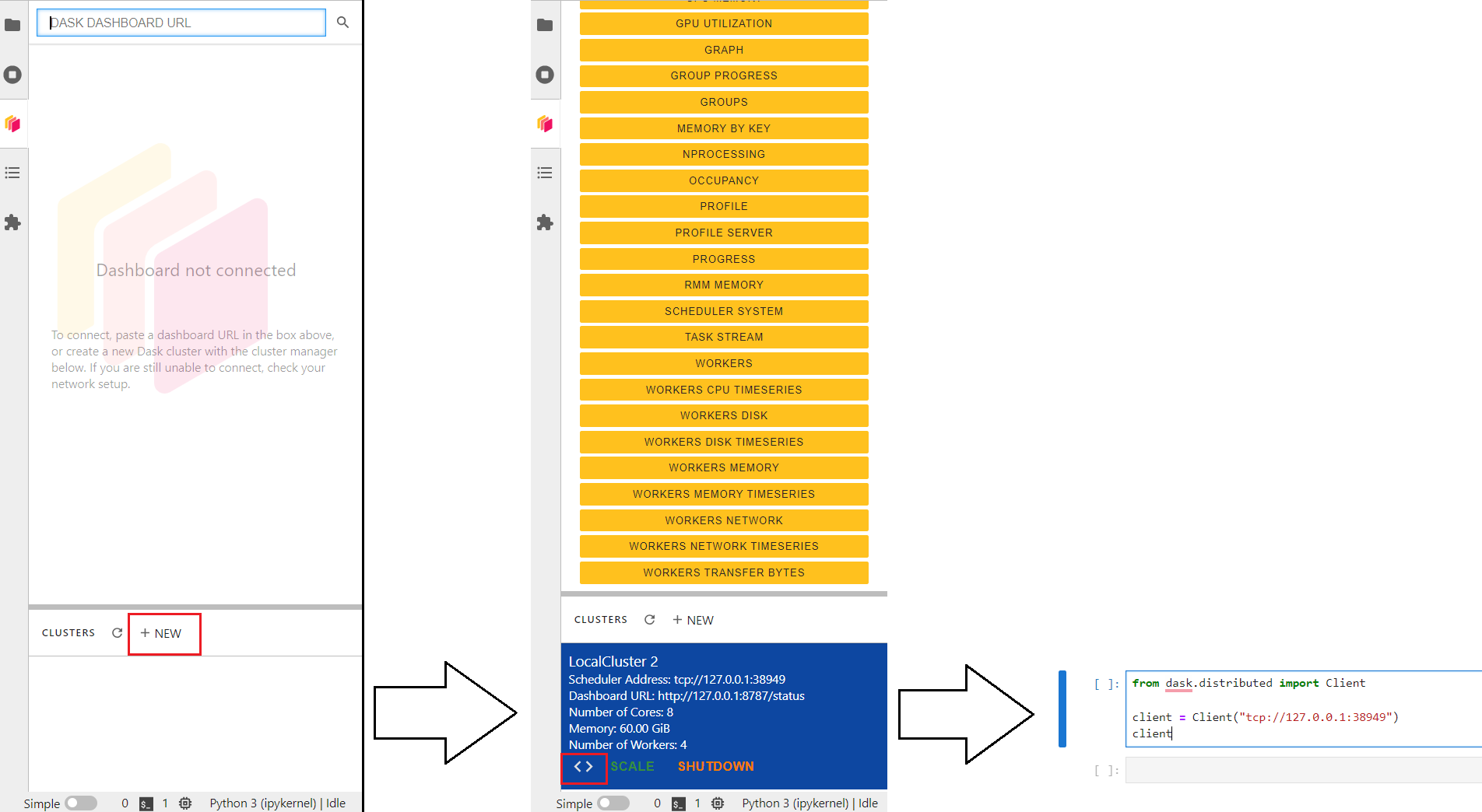
Click on Launch dashboard in Jupyter Lab to see the performance of the supercomputer.

from dask.distributed import Client

client = Client("tcp://127.0.0.1:34947")
client

Client

Client-4ec12b74-9849-11f0-9c1a-ac1f6bb2a858

Connection method: Direct
Dashboard: http://127.0.0.1:8787/status

Launch dashboard in JupyterLab

Scheduler Info

Scheduler

Scheduler-85cf634d-e240-4d65-ad38-98abe3eac49f

Comm: tcp://127.0.0.1:34947	Workers: 4
Dashboard: http://127.0.0.1:8787/status	Total threads: 8
Started: 19 minutes ago	Total memory: 64.00 GiB

Workers

Worker: 0

Comm: tcp://127.0.0.1:42295	Total threads: 2
Dashboard: http://127.0.0.1:32801/status	Memory: 16.00 GiB
Nanny: tcp://127.0.0.1:41705
Local directory: /run/nvme/job_29827827/tmp/dask-scratch-space/worker-a582it2o
Tasks executing:	Tasks in memory:
Tasks ready:	Tasks in flight:
CPU usage: 0.0%	Last seen: Just now
Memory usage: 115.53 MiB	Spilled bytes: 0 B
Read bytes: 9.08 kiB	Write bytes: 7.36 kiB

Worker: 1

Comm: tcp://127.0.0.1:33075	Total threads: 2
Dashboard: http://127.0.0.1:33043/status	Memory: 16.00 GiB
Nanny: tcp://127.0.0.1:46479
Local directory: /run/nvme/job_29827827/tmp/dask-scratch-space/worker-79vmg82q
Tasks executing:	Tasks in memory:
Tasks ready:	Tasks in flight:
CPU usage: 2.0%	Last seen: Just now
Memory usage: 114.57 MiB	Spilled bytes: 0 B
Read bytes: 9.08 kiB	Write bytes: 7.36 kiB

Worker: 2

Comm: tcp://127.0.0.1:42249	Total threads: 2
Dashboard: http://127.0.0.1:37989/status	Memory: 16.00 GiB
Nanny: tcp://127.0.0.1:38737
Local directory: /run/nvme/job_29827827/tmp/dask-scratch-space/worker-bv1widki
Tasks executing:	Tasks in memory:
Tasks ready:	Tasks in flight:
CPU usage: 2.0%	Last seen: Just now
Memory usage: 114.70 MiB	Spilled bytes: 0 B
Read bytes: 9.08 kiB	Write bytes: 7.36 kiB

Worker: 3

Comm: tcp://127.0.0.1:36423	Total threads: 2
Dashboard: http://127.0.0.1:40625/status	Memory: 16.00 GiB
Nanny: tcp://127.0.0.1:44763
Local directory: /run/nvme/job_29827827/tmp/dask-scratch-space/worker-8l8c1scr
Tasks executing:	Tasks in memory:
Tasks ready:	Tasks in flight:
CPU usage: 2.0%	Last seen: Just now
Memory usage: 115.24 MiB	Spilled bytes: 0 B
Read bytes: 8.96 kiB	Write bytes: 7.36 kiB

Read the Cell Towers using Dask

%%time

# create a Dask dataframe
world_towers = dask.dataframe.read_csv('L2-CellTowers-data.csv')

# create a Dask geodataframe
world_towers = world_towers.set_geometry(
                    	geodask.points_from_xy(world_towers, 'lon', 'lat')
                        )

CPU times: user 22.5 ms, sys: 2.2 ms, total: 24.7 ms
Wall time: 91.3 ms

type(world_towers)

dask_geopandas.expr.GeoDataFrame

world_towers.head()

	radio	mcc	net	area	cell	unit	lon	lat	range	samples	changeable	created	updated	averageSignal	geometry
0	UMTS	262	2	801	86355	0	13.285512	52.522202	1000	7	1	1282569574	1300155341	0	POINT (13.28551 52.5222)
1	GSM	262	2	801	1795	0	13.276907	52.525714	5716	9	1	1282569574	1300155341	0	POINT (13.27691 52.52571)
2	GSM	262	2	801	1794	0	13.285064	52.524000	6280	13	1	1282569574	1300796207	0	POINT (13.28506 52.524)
3	UMTS	262	2	801	211250	0	13.285446	52.521744	1000	3	1	1282569574	1299466955	0	POINT (13.28545 52.52174)
4	UMTS	262	2	801	86353	0	13.293457	52.521515	1000	2	1	1282569574	1291380444	0	POINT (13.29346 52.52152)

print(f'Total cell towers: {len(world_towers)}')

Total cell towers: 47263882

We will calculate the spatial partition of our geodataframe. We need it previously for the visualizations. If you want to know more about what methods of spatial partitions are you can check the Dask-geopandas spatial partition Documentation

# calculate spatial partitions
world_towers.calculate_spatial_partitions()

Visualization

To visualize large datasets there are already specialized tools like Pydeck and Datashader/Holoviews. The development of big data formats has advanced to new light extensions of data like Geoparquet from Pyarrow and it is integrated into a new visualization library called Lonboard which is developed for fast and interactive visualization of vector data in Jupyter.

For this example with Cell Towers we are going to explore the options with Datashader.

%%time

# canvas object
canvas = ds.Canvas(plot_width=900, plot_height=500)

# variable columns aggregation like agg=ds.max("column-name")
agg = canvas.points(world_towers, geometry='geometry', agg=ds.count())

# image shade with a distribution like ‘eq_hist’ [default], ‘cbrt’ (cube root), ‘log’ (logarithmic), and ‘linear’
# cmaps like fire, kb, kr, kg, bgyw

im = ds_function.shade(agg, cmap=cc.bmy, how="eq_hist")
ds_function.set_background(im, "#0A0A0A")

# save
export = partial(export_image, background = "#0A0A0A", export_path='output')
export(im, 'CellTowers-worldwide')

CPU times: user 2.06 s, sys: 51.5 ms, total: 2.11 s
Wall time: 2min 6s

By country

If you want to visualize the Cell Towers by country check the MCC (Mobile Country Code) for example if you want to subset only Finland you can use the MCC=244, or combine codes like Estonia 248, Sweden 240, Denmark 238, Norway 242, India 404, Germany 262, etc

%%time

# -- Choose MCC
MCC = [262]
geodata_view = world_towers.loc[world_towers.mcc.isin(MCC)].compute()

# canvas object
canvas = ds.Canvas(plot_width=500, plot_height=600)

# variable columns aggregation like agg=ds.max("column-name")
agg = canvas.points(geodata_view, geometry='geometry', agg=ds.count())

# image shade with a distribution like ‘eq_hist’ [default], ‘cbrt’ (cube root), ‘log’ (logarithmic), and ‘linear’
# cmaps like fire, kb, kr, kg, bgyw

im = ds_function.shade(agg, cmap=cc.bgyw, how="eq_hist")
ds_function.set_background(im, "#0A0A0A")

# save
export = partial(export_image, background = "#0A0A0A", export_path='output')
export(im, f'CellTowers-MCC-{MCC}')

CPU times: user 7.62 s, sys: 983 ms, total: 8.6 s
Wall time: 33.6 s

If you have been using Geopandas to read your data later on you can digest it into a Dask-GeoDataFrame using the function from_geopandas(). This method can be used when you need to do operations using distributed computing.

For now we will continue using our Dask-GeoDataFrame not ot load the same data repetitively into our memory.

Computing test

There is a particularity of the Dask-Dataframe. When you want to generate statistics or spatial operations you need to use the function compute() or it will not work. This happens because Dask generates a mapping workflow and it operates once you give the order using compute(). Let’s see some small examples and let’s monitor the HPC usage as well.

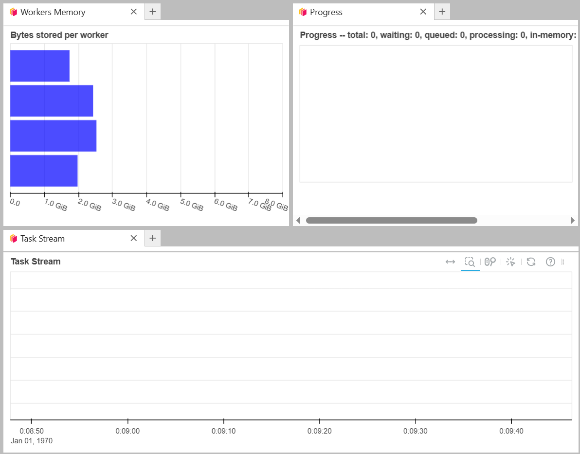
To check the resources monitoring, you can open Dask Dashboard from the initial client. If you want to know more in details about the metrics check the Dask Dashboard Documentation

Let’s see some examples of the processing with Dask. The output will be empty because there is no compute() function. Take a look.

%%time

# -- What is the average range of the Cell Towers?

world_towers.range.mean();

CPU times: user 1.04 ms, sys: 0 ns, total: 1.04 ms
Wall time: 1.05 ms

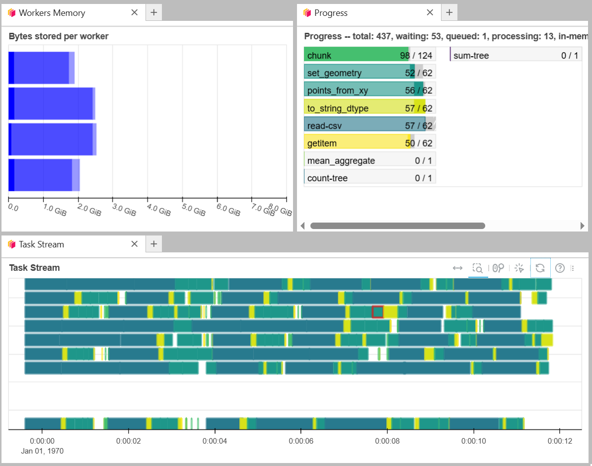
Now we will use compute() to generate the value. We will notice that it will operate for a longer time because it is running. While it is running, you can notice how the resources are being used in the Dashboard.

%%time 

# using compute
world_towers.range.mean().compute()

CPU times: user 14.1 ms, sys: 1.29 ms, total: 15.4 ms
Wall time: 15.4 s

2391.7451241732533

Metrics in Dashboard.

It will give a processed value as output.

Spatial operation test

Let’s do a spatial operation computing the number of points in a selected country. For this example, we will check the points within the ISO3=FIN for Finland.

# get iso3 geometry
iso3_geom = 'FIN'
iso3_country = world_gdf.loc[world_gdf.iso3==iso3_geom].reset_index(drop=True).at[0, 'geometry']

Using Geopandas

%%time
s = time.time()

# read with Pandas
data = pd.read_csv(r'L2-CellTowers-data.csv.gz', compression='gzip')

# create a Geodataframe
geodata = gpd.GeoDataFrame(data, 
                           geometry = gpd.points_from_xy(data.lon, data.lat),
                           crs=4326)

# -----------

# check cell towers within using compute
mcc_within_gdf = geodata.within(iso3_country)

# mask
fin_celltowers_gdf = geodata.loc[mcc_within_gdf]

# ---------------------------------------------------------
time_gpd = time.time() - s

mcc_within_gdf

CPU times: user 1min 5s, sys: 11.9 s, total: 1min 17s
Wall time: 1min 18s

0           False
1           False
2           False
3           False
4           False
            ...  
47263877    False
47263878    False
47263879    False
47263880    False
47263881    False
Length: 47263882, dtype: bool

Dask - not computed

This next process is tested only as a mapping workflow (no processing). You will notice how the output is only mapped but not executed yet.

%%time
s = time.time()

# -- Test scheduled

# check cell towers within
mcc_within = world_towers.within(iso3_country)

# mask
fin_celltowers = world_towers.loc[mcc_within]

# ---------------------------------------------------------
time_scheduled = time.time() - s

mcc_within

CPU times: user 7.48 ms, sys: 1.06 ms, total: 8.54 ms
Wall time: 9.38 ms

Dask Series Structure:
npartitions=62
    bool
     ...
    ... 
     ...
     ...
Dask Name: within, 5 expressions
Expr=UFunc(within)

Dask - computed

Then, we will use compute() to run the mapping workflow scheduled. It will give a processed output.

%%time
s = time.time()

# mask cell towers using within and compute
fin_celltowers = world_towers.loc[world_towers.within(iso3_country)].compute()

# ---------------------------------------------------------
time_compute = time.time() - s

CPU times: user 1.99 s, sys: 39.2 ms, total: 2.03 s
Wall time: 18 s

type(fin_celltowers)

geopandas.geodataframe.GeoDataFrame

len(fin_celltowers) 

260749

len(fin_celltowers_gdf)

260749

For your information, if you have a Dask-Dataframe object and you want to convert it toa Geodataframe you simply run `Dask-Object.compute()’ and it will give a Geodataframe as an output.

Let’s do the same process using only GeoDataFrames. We will notice in the HPC resources that Geopandas uses a single core.

The cell towers we are masking using within() are in the Finland border. Let’s check with Datashader

%%time

# canvas object
canvas = ds.Canvas(plot_width=400, plot_height=600)

# variable columns aggregation like agg=ds.max("column-name")
agg = canvas.points(fin_celltowers_gdf, geometry='geometry', agg=ds.count())

# image shade with a distribution like ‘eq_hist’ [default], ‘cbrt’ (cube root), ‘log’ (logarithmic), and ‘linear’
# cmaps like fire, kb, kr, kg, bgyw

im = ds_function.shade(agg, cmap=cc.kbc, how="eq_hist")
ds_function.set_background(im, "#0A0A0A")

# save
export = partial(export_image, background = "#0A0A0A", export_path='output')
export(im, f'CellTowers-MCC-within-{iso3_geom}')

CPU times: user 512 ms, sys: 0 ns, total: 512 ms
Wall time: 550 ms

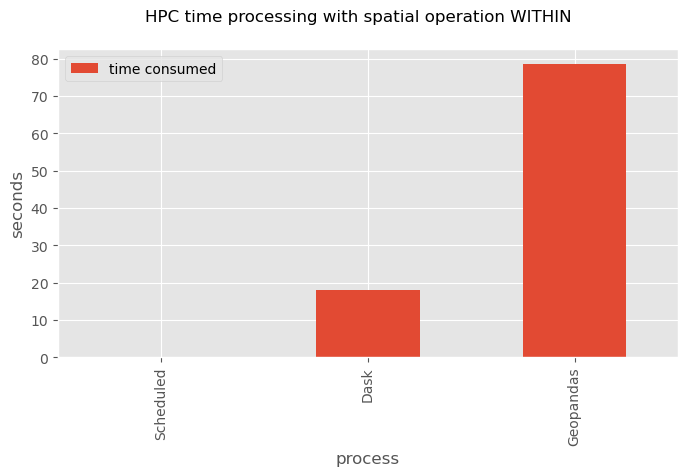
About the performance

As we expected running Dask is faster than Geopandas due to the parallel utilization of Cores.

Here is a quick view of the time process of the within spatial operation.

plt.style.use('ggplot')

# times
time_sub = pd.DataFrame({'process':['Scheduled', 'Dask', 'Geopandas'],
                         'time consumed':[time_scheduled, time_compute, time_gpd]}).set_index('process')

ax = time_sub.plot(figsize=(8, 4), kind='bar');

ax.set_ylabel('seconds')
ax.set_xlabel('process')

plt.suptitle('HPC time processing with spatial operation WITHIN');

Global Spatial Join

We are going to run the Spatial Join to all cell towers worldwide using the country’s administrative border. The comparison will be done using Dask with 8 cores and Geopandas with a single core.

Dask-Parallel

Dask-Geopandas supports only inner operation in Spatial Join and some of the cell towers were removed most probably because they were out of the country polygons.

Output: Country geometry with cell tower count.

%%time

s = time.time()

# ----- Spatial Join with dask

celltowers_dask = geodask.sjoin(world_towers, world_gdf, 
                         predicate='within', how='inner')

# count cell towers
celltowers_count = celltowers_dask.groupby('iso3').iso3.agg('count').compute()

# add cell towers count to frame
celltowers_count_df = celltowers_count.to_frame(name="towers_count")

# add geom
celltowers_borders = world_gdf.merge(celltowers_count_df, on='iso3', how='inner')


# ------------------------------------------- 
time_dask = time.time() - s

CPU times: user 72.7 ms, sys: 2.62 ms, total: 75.3 ms
Wall time: 29.5 s

celltowers_dask.head()

	radio	mcc	net	area	cell	unit	lon	lat	range	samples	changeable	created	updated	averageSignal	geometry	index_right	iso3	name	continent	cc_admin
0	UMTS	262	2	801	86355	0	13.285512	52.522202	1000	7	1	1282569574	1300155341	0	POINT (13.28551 52.5222)	188	DEU	Germany	Europe	[8, 173, 225]
1	GSM	262	2	801	1795	0	13.276907	52.525714	5716	9	1	1282569574	1300155341	0	POINT (13.27691 52.52571)	188	DEU	Germany	Europe	[8, 173, 225]
2	GSM	262	2	801	1794	0	13.285064	52.524000	6280	13	1	1282569574	1300796207	0	POINT (13.28506 52.524)	188	DEU	Germany	Europe	[8, 173, 225]
3	UMTS	262	2	801	211250	0	13.285446	52.521744	1000	3	1	1282569574	1299466955	0	POINT (13.28545 52.52174)	188	DEU	Germany	Europe	[8, 173, 225]
4	UMTS	262	2	801	86353	0	13.293457	52.521515	1000	2	1	1282569574	1291380444	0	POINT (13.29346 52.52152)	188	DEU	Germany	Europe	[8, 173, 225]

celltowers_borders.head()

	iso3	name	continent	geometry	cc_admin	towers_count
0	UGA	Uganda	Africa	MULTIPOLYGON (((33.9211 -1.00194, 33.92027 -1....	[12, 213, 204]	44169
1	UZB	Uzbekistan	Asia	MULTIPOLYGON (((70.97081 42.25467, 70.98054 42...	[221, 76, 8]	23384
2	IRL	Ireland	Europe	MULTIPOLYGON (((-9.97014 54.02083, -9.93833 53...	[8, 173, 225]	142387
3	ERI	Eritrea	Africa	MULTIPOLYGON (((40.13583 15.7525, 40.12861 15....	[12, 213, 204]	110
4	MNG	Mongolia	Asia	MULTIPOLYGON (((116.71138 49.83047, 116.64665 ...	[221, 76, 8]	7990

print(f'Total cell towers before Spatial Join: {len(world_towers)}')
print(f'Total output countries: {celltowers_borders.name.nunique()}\n')

print(f'Total Spatial Join time Dask: {round(time_dask/60, 2)} minutes')

Total cell towers before Spatial Join: 47263882
Total output countries: 225

Total Spatial Join time Dask: 0.49 minutes

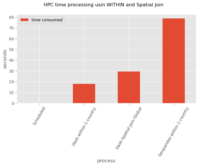
Time processing

In a comparison of Dask and Geopandas we can see that Dask operates faster and uses the HPC resources efficiently. On the other hand, Geopandas takes longer time processing 1 country than Dask processing at global level (225 countries)

plt.style.use('ggplot')

# times
time_sub = pd.DataFrame({'process':['Scheduled', 'Dask-within-1-country',  'Dask-Spatial-Join-Global', 'Geopandas-within-1-country',],
                         'time consumed':[time_scheduled, time_compute, time_dask, time_gpd ]}).set_index('process')

ax = time_sub.plot(figsize=(8, 4), kind='bar');

ax.set_ylabel('seconds')
ax.set_xlabel('process')

plt.xticks(rotation = 60)
plt.suptitle('HPC time processing usin WITHIN and Spatial Join');

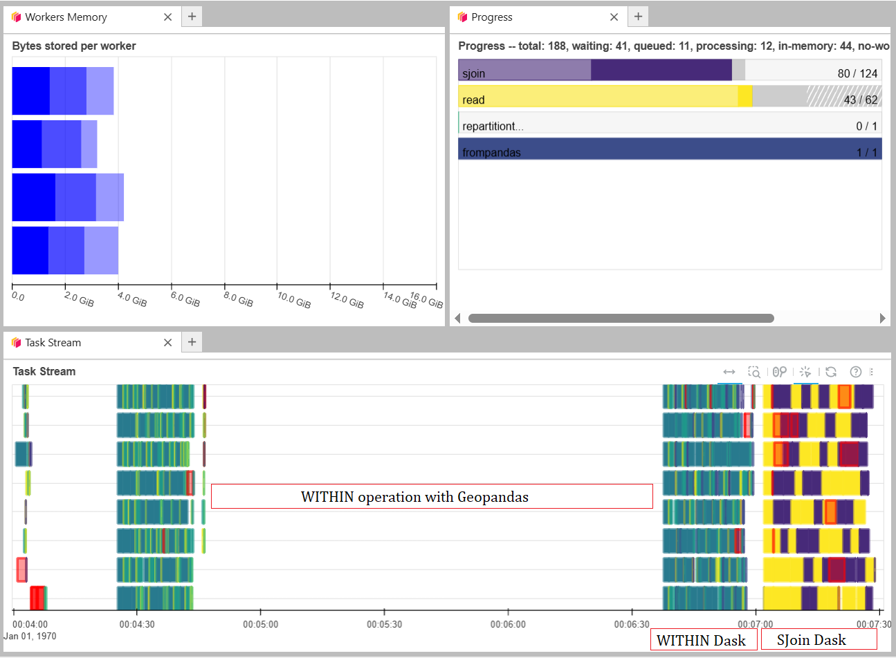
Parallelization monitoring

The Dask Dashboard shows the processing in parallel. In the next image, you can see how the Within operation with Geopandas is not using distributed computing meanwhile Within with Dask is distributing the computation. Also, in yellow, you can see how the Spatial Join with Dask runs in parallel.

Geopandas-single core

Unfortunately, when running the Spatial Join with Geopandas the process runs out of memory. Geopandas uses the memory gradually in the spatial join and when reaching the limit in Puhti it breaks the connection.

If you try you will find a message after the connection breaks.

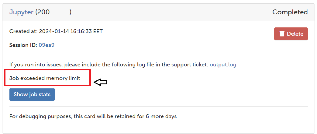
So, it shows how efficiently Dask-Geopandas can operate using parallelization. Sorry, Geopandas.

Note!

If you want to measure the time processing using Geopandas you can operate spatial join in a loop, per country, it will take quite long processing time. This approach was avoid to give a clear and fast view of Parallelization with Dask-Geopandas

Country visualization

Let’s give a quick view to the output of the Spatial Join - Per country border (Tower count)

# add a category column
celltowers_borders["cat"] = celltowers_borders["iso3"].astype("category")

celltowers_dask.dtypes

radio            string[pyarrow]
mcc                        int64
net                        int64
area                       int64
cell                       int64
unit                       int64
lon                      float64
lat                      float64
range                      int64
samples                    int64
changeable                 int64
created                    int64
updated                    int64
averageSignal              int64
geometry                geometry
index_right                int64
iso3             string[pyarrow]
name             string[pyarrow]
continent        string[pyarrow]
cc_admin         string[pyarrow]
dtype: object

%%time

# canvas object
canvas = ds.Canvas(plot_width=900, plot_height=500)

# variable columns aggregation like agg=ds.max("column-name")
agg = canvas.polygons(celltowers_borders, geometry='geometry', agg=ds.max('towers_count'))

# image shade with a distribution like ‘eq_hist’ [default], ‘cbrt’ (cube root), ‘log’ (logarithmic), and ‘linear’
# cmaps like fire, kb, kr, kg, bgyw

im = ds_function.shade(agg, cmap=cc.blues, how='eq_hist')

ds_function.set_background(im, "white")

# save
export = partial(export_image, background = "white", export_path='output')
export(im, 'CellTowers-agg-worldwide-countries')

CPU times: user 2.82 s, sys: 49.9 ms, total: 2.87 s
Wall time: 2.9 s

Spatial Join per region

You can also get the output of the Spatial Join using the Cell Tower layer. To save resources and time during the process we are going to selecte specific countries per region. In the next lines, you will find the spatial join using a selected group of countries.

Output: Cell Towers with attribute of country (Cell Towers layer)

Europe

%%time

# -- create a spatial join with desired countries

# subset world towers

# -- Choose MCC
MCC = [244, 240, 242, 238, 248, 247, 246, 262, 260, 362, 274, 214, 208, 222, 268, 206, 232, 228, 230]
world_towers_subset = world_towers.loc[world_towers.mcc.isin(MCC)]

# ---- spatial join

celltowers_dask_vis = geodask.sjoin(world_towers_subset, world_gdf, 
                                     predicate='within', how='inner').compute()

# add a category column
celltowers_dask_vis["cat"] = celltowers_dask_vis["iso3"].astype("category")

CPU times: user 4.79 s, sys: 3.15 s, total: 7.94 s
Wall time: 57.5 s

%%time

# canvas object
canvas = ds.Canvas(plot_width=700, plot_height=800)

# variable columns aggregation like agg=ds.max("column-name")
agg = canvas.points(celltowers_dask_vis, geometry='geometry', agg=ds.count_cat('cat'))

# image shade with a distribution like ‘eq_hist’ [default], ‘cbrt’ (cube root), ‘log’ (logarithmic), and ‘linear’
# cmaps like fire, kb, kr, kg, bgyw
im = ds_function.shade(agg, color_key=cc.glasbey_light)

ds_function.set_background(im, "#0A0A0A")

# save
export = partial(export_image, background = "#0A0A0A", export_path='output')
export(im, 'CellTowers-cat-EU-countries')

CPU times: user 24.8 s, sys: 2.28 s, total: 27.1 s
Wall time: 27.2 s

South America

%%time

# -- create a spatial join with desired countries

# subset world towers

# -- Choose MCC
MCC = [740, 732, 716, 730, 722, 724, 748, 744, 734]
world_towers_subset = world_towers.loc[world_towers.mcc.isin(MCC)]

# ---- spatial join

celltowers_dask_vis = geodask.sjoin(world_towers_subset, world_gdf, 
                                     predicate='within', how='inner').compute()

# add a category column
celltowers_dask_vis["cat"] = celltowers_dask_vis["iso3"].astype("category")

CPU times: user 5.29 s, sys: 967 ms, total: 6.26 s
Wall time: 31.4 s

%%time

# canvas object
canvas = ds.Canvas(plot_width=700, plot_height=700)

# variable columns aggregation like agg=ds.max("column-name")
agg = canvas.points(celltowers_dask_vis, geometry='geometry', agg=ds.count_cat('cat'))

# image shade with a distribution like ‘eq_hist’ [default], ‘cbrt’ (cube root), ‘log’ (logarithmic), and ‘linear’
# cmaps like fire, kb, kr, kg, bgyw
im = ds_function.shade(agg, color_key=cc.glasbey_light)

ds_function.set_background(im, "#0A0A0A")

# save
export = partial(export_image, background = "#0A0A0A", export_path='output')
export(im, 'CellTowers-cat-SA-countries')

CPU times: user 6.62 s, sys: 354 ms, total: 6.97 s
Wall time: 6.98 s