Lesson 2. Shortest Path#
Shortest Path (Dijkstra’s) in OSM driving network between residential buildings and Rautatieasema#
Introduction#
In this Lesson, we are going to process the Shortest Path between every building registered in OpenStreetMap (OSM) to the Central Railway Station in Helsinki. This practice gives an overview about the accessibility of the population to the Helsinki city center considering the central railway station as the central point. The Dijkstra’s algorithm can be applied in the OSM driving network using the Python library OSMnx which operates network analysis under the hood using NetworkX. The newest version of OSMnx implements Core Parallelization so we can operate the routing in parallel in the available cores of your machine.
This exercise is designed for teaching purposes of Spatial Data Science with High Performance Computing (HPC) at Aalto University. Thanks to the computational resources provided by CSC this exercises was tested in the Puhti supercomputer.
Objective#
To compare the advantage of processing time of Shortest Path algorithm in the Helsinki Region using parallel computing
Datasets#
Both datasets are fetched during the workflow from OSM using the OSMnx and they are:
Buildings footprint in the main central area of Helsinki Region (at x Km radius)
Central railway station - Rautatieasema
Output#
The process gives as output a layer with all the routes from every buildings in the Helsinki Region to the Rautatieasema
Find the a map of the results at the beginning of this notebook
Limitation#
In this example, if you define a small radius the study area will fetch a small amount of buildings and then the number of shortest paths computed will be small.
Attention
If you compute less than ~2000 shortest path will take longer time processing in Parallel than with a single core. The benefit of using Parallelization start when you compute over ~5000 shortest paths
HPC resources#
CSC Machine-Puhti:
Partition: small
CPU Cores: 8
Memory (GB): 32
Local Disk (GB): 60
Hands-on coding#
Follow the instructions and run every cell in the supercomputer.
Importing Python libraries#
Be sure that you have installed the OSMnx>=1.6.0 in your environment. Get familiar with this library reading a bit the OSMnx Documentation
# -- for (geospatial) analysis
import geopandas as gpd
from shapely.geometry import MultiLineString
from shapely import ops
import osmnx as ox

import pandas as pd

# -- visualization
import matplotlib.pyplot as plt

# -- for optimization of computational resources
from joblib import Memory
import multiprocessing as mp

# -- folders
import os
import glob

# -- time processing
import time
import warnings
warnings.filterwarnings('ignore')
We are going to create a folder output where the results are going to be stored
# results folder
if not os.path.exists('output'):
    os.makedirs('output')
Fetch Central Railway Station#
We will fetch the location of Ratatieasema from OSM using geocoding. Then, we are going to define a certain radius from the Central Railway Station as our study area. The process in a small area will show the benefits of using parallelization in a short processing time. If you are are willing to check a long run example feel free to test this notebook using a large radius. For example, 200 km.
Using OSMnx we can geocode location with the function geocoder.geocode_to_gdf(). We will define a function to simplify the process.
def get_Rautatieasema_gfd():
    '''
    Give back Rautatori Point geometry in WGS84 from OSM
        Return Point geometry
    '''
    # Geocode the address
    station = ox.geocoder.geocode_to_gdf("Helsinki Central Railway station")

    # reset index
    station = station.reset_index(drop=False)
    station = station[['name', 'geometry']]

    # get centroid - avoid warning getting the centroid in local CRS for more accuracy
    station['geometry'] = station.to_crs(3067).centroid.to_crs(4326)

    return station
We will use the function to the Rautatieasema location as a geodataframe. Then, we will make a copy to transform into a polygon for the study area.
# fetch rautatieasema as geodataframe
rautatieasema = get_Rautatieasema_gfd()

# make a copy for study area
study_area = rautatieasema.copy()
Radius of study area#
Add a desired radius for defining the study area. The radius defined will create a circle using the Central Railway Station as the center. By default, a good example can be seen using a radius of 10 Km (10 000 meters). Lowest radius shows not significant benefit and bigger radius causes long processing time. We want to keep it a modest short time for educational purposes.
RADIUS = 10000 # <---- meters --- add a radius

# create study area geometry using crs 3067 (Finnish crs)
study_area.geometry = study_area.geometry.to_crs(3067).buffer(RADIUS).to_crs(4326)
Let’s visualize the study area.
# visualize study area
study_area.explore()
Fetch OSM residential buildings#
To fetch OSM features it is necessary to have two elements: 1) and OSM defined area like and Administrative Unit, and 2) a tag for the element we want to fetch. Check the next links to understand a bit the areas you can fetch and tags you can find. When using OSM defined reas from Nominatim you need to use the function features_from_place(). For this exercise, we will fetch using a defined study area using the function features_from_polygon().
Take a look at the available OSM areas in the Nominatim website and the tags for features in the OSM Wiki website.
Explore a bit more the options you have using the tags. For example, what if you include only apartment buildings? or only houses? Both?
# ------> Fetch residential buildings

# get geometry of Rautatieasema
place_geom = study_area.geometry[0]

# Tags for residential buildings
tags = {'building': 'residential'}

# run
all_buildings = ox.features_from_polygon(place_geom, tags)
Once you have fetched the buildings you will see that it contains double index and many columns. We will simplify this to have a more kneat frame of the data simple by deleting the indexes and keeping only the street name and the geometry.
# ------> Reset index and get street name

all_buildings = all_buildings.reset_index(drop=False)
all_buildings = all_buildings[['osmid', 'addr:street', 'geometry']]

# rename
all_buildings = all_buildings.rename(columns={'addr:street':'street_name'})
The geometry of the buildings are represented by points and polygons. What we need to have is only points because the Shortest Path analysis runs between two points (longitude and latitude) so we will add the centroid of every geometry to remove the polygons and keep them as centroids.
# fix geometries using centroids
all_buildings['geometry'] = all_buildings['geometry'].apply(lambda geom: geom.centroid)
Here is a quick view of the buildings data.
print(f'In total {len(all_buildings)}')

all_buildings.head()
In total 5291
| osmid | street_name | geometry | |
|---|---|---|---|
| 0 | 930663425 | Marjatie | POINT (24.98284 60.25331) |
| 1 | 4266889 | Servin Maijan tie | POINT (24.83679 60.19060) |
| 2 | 15505174 | Karhutie | POINT (25.03614 60.20457) |
| 3 | 15505279 | Karhutie | POINT (25.03645 60.20501) |
| 4 | 15505332 | Karhutie | POINT (25.03642 60.20482) |
Let’s use explore() to see our buildings.
print(f'Total residential buildings: {len(all_buildings)}')

all_buildings.explore(color='red',
                      tiles='CartoDB positron',
                      marker_kwds={'radius':4, 'alpha':0.6},
                      style_kwds={'stroke':False})
Total residential buildings: 5291
Prepare Origins as a List#
The Shortest Path function in OSMnx can process A-Origin to A-Destination. A particularity of this function is that you can process pair routes as Lists in a way that [A-Origin, B-Origin, C-Origin, ...] to [A-Destination, B-Destination, C-Destination, ...] will give [A-OD, B-OD, C-OD, ...].
Based on this feature of the OSMnx library we are going to start organizing a List all_origins that contains geometry objects of every building we have fetched from OSM in the Helsinki Region.
# --------> define origin List

# list
all_origins = []

for row in all_buildings.itertuples(index=True):

    # tuple, only geometries
    geom = row.geometry

    all_origins.append(geom)
all_origins[:5]
[<POINT (24.983 60.253)>,
 <POINT (24.837 60.191)>,
 <POINT (25.036 60.205)>,
 <POINT (25.036 60.205)>,
 <POINT (25.036 60.205)>]
Fetching road network#
In this step we are going to fetch the Graph object containing the edges (roads) and nodes (intersections) of the OSM driving network. As we are using a defined study the function that we will use is the graph_from_polygon() from OSMnx. In case you want to fetch administrative border you might need to use the function graph_from_place()
Note!
We are going to create a function that packs the OSMnx function. The objective is to add it to cache memory to optimize memory resources every time you re run this notebook.
The library joblib is able to cache processes that can be repetitive and optimize the memory in a workflow. This means, that the first time you fetch the Graph from OSM will take some time, but the next times will be quick because the process is cached.
def graph_Helsinki(place_geom, network_type='drive'):
    '''
    Packed function for repetitive running and testing

    - place_geom: geom, area defined
    - network_type: string, type of OSM network from drive, bike, walk

        return <Function>
    '''

    return ox.graph_from_polygon(place_geom, network_type)
Cache the Graph fetch
# cache
memory = Memory('cache', verbose=0)
graph_Helsinki_cached = memory.cache(graph_Helsinki)
%%time

# get the road network as graph object
graph = graph_Helsinki_cached(place_geom, network_type='drive')
CPU times: user 15.4 s, sys: 242 ms, total: 15.6 s
Wall time: 17.1 s
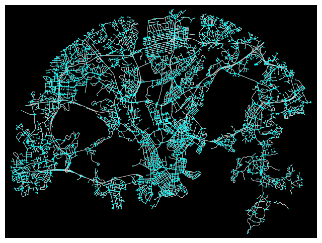
The OSMNX can plot the graph using the function plot_graph(). We added some modifications to have a clean view.
fig, ax = ox.plot_graph(graph,
                        node_size=2,
                        node_color='cyan',
                        edge_linewidth=0.4,
                        edge_color='white',
                        bgcolor='black')
Prepare Destination as Geometry#
We have fetched already the location of Rautatieasema as a geodataframe using the function get_Rauratientori_gfd(). We will store the geometry object in a variable called destin_geom.
We will require simply the geometry object when routing the Shortest Path.
Let’s have a quick visualization of the location of Rautatieasema.
# Rautatiesema

# geom
destin_geom = rautatieasema.geometry[0]

rautatieasema.explore(color='magenta',
                      marker_kwds={'radius':50, 'alpha':0.8})
A. Shortest Path - Parallelization#
We are going to run step by step the process of finding the Shortest Path using Parallelization. The advantage we have separating the workflow step by step is that we are able to run in parallel specific parts of the Shortest Path and it saves processing time.
About the Core Parallelization#
To start understanding a bit more the parallel computing let’s take a look the available resources in our machine using the next command.
!lscpu | egrep 'Model name|Socket|Thread|NUMA|CPU\(s\)'
CPU(s):              40
On-line CPU(s) list: 0-39
Thread(s) per core:  1
Socket(s):           2
NUMA node(s):        2
Model name:          Intel(R) Xeon(R) Gold 6230 CPU @ 2.10GHz
NUMA node0 CPU(s):   0-19
NUMA node1 CPU(s):   20-39
We can see the number of Cores available in the CPU(s) sections. The partition contains in total 40 Cores (depends the partition machine in this case was small) but the configuration we specified at the beginning in the machine was 8 Cores or any other number. So? Despite 40 cores are available only 8 cores are reserved for our analysis.
We can monitor our processes and the Core utilization with htop library that let us visuallize dinamically how the computer is using the resources. If you are willing to monitor your process you should open in a new command line $ htop (be sure you are using your own environment)
Let’s take a look at the resources utilization after each process.
A1. Nearest destination nodes#
The Shortest Path is operated in the OSM network between nodes (intersections) so the Origin and Destination location are simply a reference that helps to find the closest node where the routing should start.
In the next cells we are going to find the closest nodes using the function nearest_nodes() from OSMNX.
The Destination is only one geometry of Rautatieasema and it requires only 1 nearest node. Additionally, the process of finding the closest node of every Origin was parellized using the library multiprocess because it contains many points.
We are going to start measuring the processing time using simple time variables at the beginning and end of the cell and we will sum up at the end to compare how the efficiency improves using parallel computation.
s = time.time()

# ---- Closest destination nodes

closest_target_node = ox.nearest_nodes(G=graph,
                                       X=destin_geom.x,
                                       Y=destin_geom.y)


# --------------------------------------------------------
d1 = time.time() - s
print(f' - Closest destination node: {d1} seconds')
- Closest destination node: 0.041275739669799805 seconds
If you can monitor the processes using htop (optional) you will see that we have in total 40 Cores. Some of them are already in use but there are still 16 Cores available for our use.
This is how the resource utilization looks if you are running the Destination node cell

As we are running a normal process the computer is using a single node: the Core #30.
A2. Nearest origin nodes#
We have many origins that we should compute and find the closest node. To optimize the time processing we are going to parallelize for every origin.
We will use the Python library multiprocess to parallelize the closest node process of the origins. Let’s start packing the function nearest_nodes() from OSMNX.
print(f'- Processing total routes: {len(all_origins)}')
- Processing total routes: 5291
def get_nearest_node(graph, geom):
    '''
    Packed function to return a closest node from geometry

    - graph: graph, osm object
    - origin_geom: point geom, individual

        return:: int, a node code
    '''

    # calculate node
    node = ox.nearest_nodes(G=graph, X=geom.x, Y=geom.y)

    return node
The multiprocess library is able to send a job to every core and optimize the workflows. The step is simple once we have packed the function we are going to use in this case get_nearest_node()
Note!
As a condition, you should be able to loop over the inputs otherwise the process is not going to be parallelized. We are looping over every origin so we can distribute the process in every core.
The variables involved in the parallelization are:
cpus: the number of cores available for computation withcpu_count()args: the parameters of our packed function, looping over every inputpool: a pool opened for every available core where asyncronize the process withstarmap_async()get(): catch the result of every process in every core and save in a list
Then, you to close the pool you close() and join().
s = time.time()

# ----- A2) Closest origins node

# get cores
cpus = mp.cpu_count()

# ----- args

args = ((graph, geom) for geom in all_origins)

# ----- pool - with function

pool = mp.Pool(cpus)
sma = pool.starmap_async(get_nearest_node, args)

# ----- get list of results

closest_origin_node_list = sma.get()
pool.close()
pool.join()


# ----------------------------------------------------------
d2_parallel = time.time() - s
print(f' - Closest node of origins [PARALLELIZED]: {d2_parallel/60} minutes')
- Closest node of origins [PARALLELIZED]: 0.9805782357851665 minutes
If you monitor the process in htop you will notice how the resource utilization changed. (This example with 16 cores)
At first you will see how the Cores start to be used:

Finally, it will occupy the 16 Cores available:

In total 16 Cores: from Core #20 to Core #35
A3. Finding Shortest Paths#
The OSMnx library has implemented the Shortest Path algoritm using the function shortest_path(). A particularity of this function is that it create routes based on OD paired-list. For example, if your input is Origins=[O1, O2, O3] and Destinations=[D1, D2, D3], the output paths are going to be defined as [O1 to D1, O2 to D2, O3 to D3].
Based on this, we need to have two lists with the same length. As we are using only 1 destination, we will multiply by the length of the origins so we have all routes to the same destination.
Fortunately, the OSMnx library has implemented in the function a parallelization parameter cpus. If you want to use all available cores, in this case 8 cores, you need to add cpus=None and it will use all available resources.
Follow the next code.
s = time.time()

# ---- target nodes should be same length as origins

closest_target_node_list = [closest_target_node] * len(closest_origin_node_list)

# -------- Shortest Path ---------

# run
routes = ox.shortest_path(graph,
                         orig = closest_origin_node_list,
                         dest = closest_target_node_list,
                         weight = 'length',
                         cpus = None) # none takes all cores, default=1


# --------------------------------------------------------------------------

d3_parallel = time.time() - s
print(f' - Shortest Path run [PARALLELIZED]: {d3_parallel/60} minutes')
- Shortest Path run [PARALLELIZED]: 0.9271456917126973 minutes
As we explained, the routes are defined between nodes, and might be the case that some nodes are too close or the origins are not connect to the network (like islands) so there are no existing routes and in those cases the OSMnx return a None object.
In this line we are going to remove the invalid routes.
# remove None values from invalid routes
all_routes = [value for value in routes if value != None]

# check routes length
len(all_routes)
5291
A4. From nodes to paths#
The output of the Shortest Path is a list of node’s codes that construct the route we want. Then, we need to extract the line geometries using those nodes.
Be aware that we can do this work using the already implemented function in OSMnx utils_graph.route_to_gdf(). Particularly, it will give a row for each route segment and it will create quite many routes for all the routes we are working on. So, we will create a function nodes_to_path() that will transform routes into a single line geometry.
Get familiar with the function.
def nodes_to_path(graph, route_nodes):
    '''
    Function to transform node's path to a single line geometry
    - graph: osm graph object
    - route_nodes: list, nodes of path
        return geodataframe with a single row
    '''

    # get route from nodes - get only geom and length
    shortest_route_parallel = ox.utils_graph.route_to_gdf(graph, route_nodes, weight='length')[['length', 'geometry']].reset_index(drop=True)

    # join the road segments
    multi_line = MultiLineString([linegeom for linegeom in shortest_route_parallel.geometry])
    total_length = sum([value for value in shortest_route_parallel['length']])

    merged_line = ops.linemerge(multi_line)

    # new gdf
    shortest_route_merged = gpd.GeoDataFrame(columns=['geometry'], geometry='geometry', crs=4326)
    shortest_route_merged.at[0, 'geometry'] = merged_line
    shortest_route_merged.at[0, 'length'] = total_length

    return shortest_route_merged
Then, we will use again a pool from multiprocess to parallelize this path geometry creation. You can monitor also the core usage using the htop
s = time.time()

# --------- A.4) Get path as geom GDF

# get cores
cpus = mp.cpu_count()

# ----- args

args = ((graph, route_nodes) for route_nodes in all_routes)

# ----- pool - with function

pool = mp.Pool(cpus)
sma = pool.starmap_async(nodes_to_path, args)

# ----- get list of results - GDF

shortest_path_gdf_list = sma.get()
pool.close()
pool.join()

# --------------------------------------------------------------------------

d4_parallel = time.time() - s
print(f' - Nodes to path: {d4_parallel/60} minutes')
- Nodes to path: 0.9617520650227864 minutes
The output will be a list of Shortest Paths stored in the variable shortest_path_gdf_list. We will gather all results into one geodataframe using concat() function.
# ------  create a single GDF

all_routes_gdf = pd.concat(shortest_path_gdf_list)
We have got the length of every route fetching the same column from OSM that probably was calculated at global level. We would like to calculate a more accurate distance computed in a Finnish CRS (3067) so we need to operate a new column and add the newly measured distance.
We will create a function.
def compute_fin_distance(shortest_path_gdf):
    '''
    Compute distance in FinCRS EPSG:3067

    - shortest_path_gdf: geodataframe, with geometry colum
        return geodataframe, with additional distance column

    '''

    # project WGS84 to EPSG3067
    distances = shortest_path_gdf.to_crs("EPSG:3067").geometry.length

    # add
    shortest_path_gdf['distance_fincrs'] = distances

    return shortest_path_gdf
# ----- Compute distance EPSG FIN

route_distance_gdf = compute_fin_distance(all_routes_gdf)
A5. Results#
We are going to check how our final geodataframe looks like and count how many routes we have calculated in total.
We will see that there is a slightly difference with distances calculated in the Finnish CRS. If you are going to use this process to calculate statistics it is recommended to do it using the distances from the local CRS.
print(f' - In total {len(all_routes_gdf)} routes processed using 8 cores\n')

route_distance_gdf.head()
- In total 5291 routes processed using 8 cores
| geometry | length | distance_fincrs | |
|---|---|---|---|
| 0 | LINESTRING (24.98252 60.25363, 24.98266 60.253... | 11722.834 | 11749.086070 |
| 0 | LINESTRING (24.83813 60.19089, 24.83812 60.190... | 9876.080 | 9902.498971 |
| 0 | LINESTRING (25.03655 60.20408, 25.03647 60.203... | 7783.723 | 7804.965027 |
| 0 | LINESTRING (25.03631 60.20566, 25.03643 60.205... | 7970.705 | 7992.303020 |
| 0 | LINESTRING (25.03655 60.20408, 25.03647 60.203... | 7783.723 | 7804.965027 |
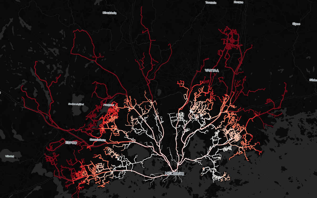
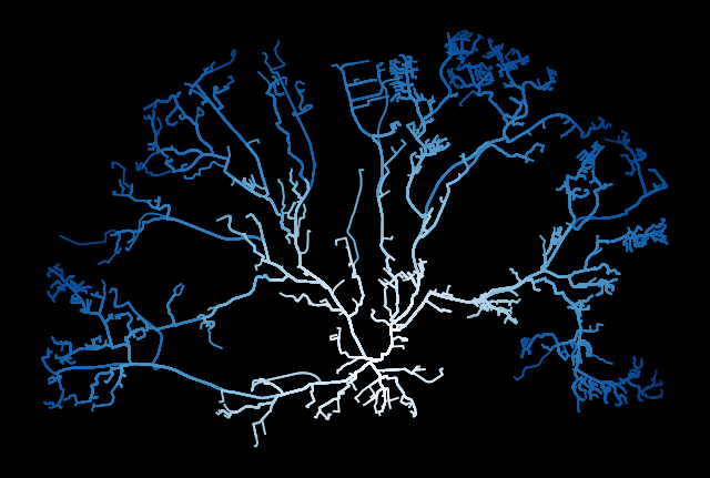
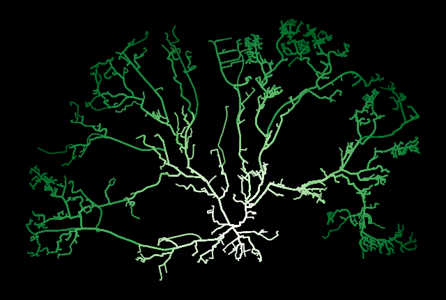
A quick plot to visualize the routes.
# sort values for visualization
all_routes_gdf = all_routes_gdf.sort_values('distance_fincrs', ascending=False)
A visualization using matplotlib
# define a style for the map
plt.style.use('dark_background')

# Plot

# routes
ax = all_routes_gdf.plot(figsize=(8, 8),
                         column='distance_fincrs',
                         linewidth=1.4,
                         cmap='Blues',
                         alpha=1,
                         zorder=1
                        );

# remove coordinates
ax.axis('off');

plt.savefig('output/shortest_path_parallel_8_core.png', dpi=300)
Finally, we are going to save in our local disk the routes as GIS format. Geopackage in this case.
s = time.time()

# -------- Save

filepath = 'output/shortest_path_parallel.gpkg'
all_routes_gdf.to_file(filepath, index=False)

# --------------------------------------------------------------------------

dsave1 = time.time() - s
print(f' - Saving time: {dsave1} seconds')
- Saving time: 1.9171314239501953 seconds
B. Shortest Path - Single Core#
Do I have to configure 1 Core?#
No, the process by default is run in a single Core, as it was run in a personal laptop. But, in this section there are not modification in the code so parallelization is not active.
B1. Nearest destination nodes#
As we have already calculated the closest node of the destination we will run only the closest node calculation for the origins, but this time using a single core.
This process we have already done only for Rautatieasema and it is store in the variable closest_target_node
closest_target_node
25413719
B2. Nearest origin nodes#
We will find the Origins nodes as a list using a single core
s = time.time()

# ----- A2-non) Closest origins node

closest_origin_node_list = [ox.nearest_nodes(G=graph,
                                           X=origin_geom.x,
                                           Y=origin_geom.y)
                               for origin_geom in all_origins]

# ----------------------------------------------------------

d2_non = time.time() - s

print(f' - Closest node of origins [NON-PARALLELIZED]: {d2_non/60} minutes')
- Closest node of origins [NON-PARALLELIZED]: 4.883958788712819 minutes
B3. Finding Shortest Paths#
Then we will run the shortest path using a single core.
s = time.time()

# ---- target nodes should be same length as origins

closest_target_node_list = [closest_target_node] * len(closest_origin_node_list)

# -------- Shortest Path ---------

# run
routes = ox.shortest_path(graph,
                         orig = closest_origin_node_list,
                         dest = closest_target_node_list,
                         weight = 'length',
                         cpus = 1)


# --------------------------------------------------------------------------

d3_non = time.time() - s
print(f' - Shortest Path run [NON-PARALLELIZED]: {d3_non/60} minutes')
- Shortest Path run [NON-PARALLELIZED]: 1.9792736689249675 minutes
We will remove non valid routes and check how many are valid.
# remove None values from invalid routes
all_routes = [value for value in routes if value != None]

# check routes length
len(all_routes)
5291
B4. Nodes to path#
The nodes to path are computed in this part with a single core.
Beforehand, the results were gathered in a list using pool from parallelization. But now, we are going to loop over each path (as nodes) and use the function previously created that return a single line geometry. On the fly, we will calculate the distance using the Finnish CRS.
Finally, we will have a single geodataframe with all routes.
s = time.time()

# --------- B.4) Get path as geom GDF

all_routes_gdf = gpd.GeoDataFrame()

for each_route in all_routes:

    # ----- create nodes path to GDF
    route_gdf = nodes_to_path(graph, each_route)

    # ----- Compute distance

    route_distance_gdf = compute_fin_distance(route_gdf)

    all_routes_gdf = pd.concat([all_routes_gdf, route_distance_gdf])

# --------------------------------------------------------------------------

d4_non = time.time() - s
print(f' - Nodes to path and distances: {d4_non/60} minutes')
- Nodes to path and distances: 2.075392679373423 minutes
B5. Results#
Let’s take a look at the results.
print(f' - In total {len(all_routes_gdf)} routes processed with 1 core\n')

all_routes_gdf.head()
- In total 5291 routes processed with 1 core
| geometry | length | distance_fincrs | |
|---|---|---|---|
| 0 | LINESTRING (24.98252 60.25363, 24.98266 60.253... | 11722.834 | 11749.086070 |
| 0 | LINESTRING (24.83813 60.19089, 24.83812 60.190... | 9876.080 | 9902.498971 |
| 0 | LINESTRING (25.03655 60.20408, 25.03647 60.203... | 7783.723 | 7804.965027 |
| 0 | LINESTRING (25.03631 60.20566, 25.03643 60.205... | 7970.705 | 7992.303020 |
| 0 | LINESTRING (25.03655 60.20408, 25.03647 60.203... | 7783.723 | 7804.965027 |
# sort values for visualization
all_routes_gdf = all_routes_gdf.sort_values('distance_fincrs', ascending=False)
With maptplotlib
# define a style for the map
plt.style.use('dark_background')

# Plot

# routes
ax = all_routes_gdf.plot(figsize=(8, 8),
                         column='distance_fincrs',
                         linewidth=1.4,
                         cmap='Greens',
                         alpha=1,
                         zorder=1
                        );

# remove coordinates
ax.axis('off');

plt.savefig('output/shortest_path_parallel_1_core.png', dpi=300)
We will save the results.
s = time.time()

# -------- Save

filepath = 'output/shortest_path_parallel.gpkg'
all_routes_gdf.to_file(filepath, index=False)

# --------------------------------------------------------------------------

dsave2 = time.time() - s
print(f' - Saving time: {dsave2} seconds')
- Saving time: 5.688600063323975 seconds
Summary#
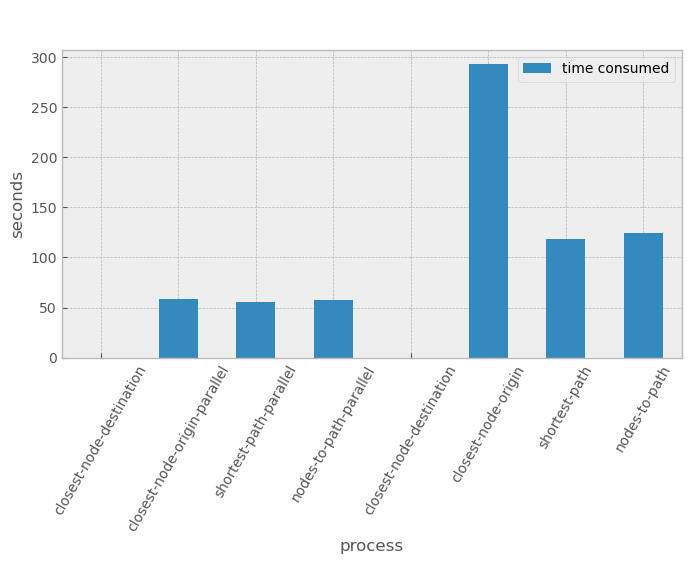
We are going to print the sum of all processing times and compare how benefitial was to use the parallelization. Be aware that:
d1corresponds to the closest node of destination ()d2corresponds to the closest node of origins (buildings)d3corresponds to the shortest path calculationd4corresponds to the transformation from nodes to line geometry
print(f'--------------------- PROCESSING TIME --------------------\n')

total_parallel = d1 + d2_parallel + d3_parallel + d4_parallel

print(f'--> Total parallel time : {round(total_parallel/60, 2)} mins -> 8 Core')

total_non = d1 + d2_non + d3_non + d4_non

print(f'--> Total time : {round(total_non/60, 2)} mins -> 1 Core')

print(f'\n--------------------- TIME PROCESSING BENEFIT --------------------\n')

print(f'--> % of improvement : {round(((total_non-total_parallel)/total_non)*100, 1)}%')
print(f'--> n paths : {len(all_routes_gdf)} at radius {RADIUS} m')
--------------------- PROCESSING TIME --------------------

--> Total parallel time : 2.87 mins -> 8 Core
--> Total time : 8.94 mins -> 1 Core

--------------------- TIME PROCESSING BENEFIT --------------------

--> % of improvement : 67.9%
--> n paths : 5291 at radius 10000 m
plt.style.use('bmh')

# times
time_sub = pd.DataFrame({'process':['closest-node-destination',
                                    'closest-node-origin-parallel',
                                    'shortest-path-parallel',
                                    'nodes-to-path-parallel',
                                    'closest-node-destination',
                                    'closest-node-origin',
                                    'shortest-path',
                                    'nodes-to-path'],
                         'time consumed':[d1,
                                          d2_parallel,
                                          d3_parallel,
                                          d4_parallel,
                                          d1,
                                          d2_non,
                                          d3_non,
                                          d4_non]}).set_index('process')

ax = time_sub.plot(figsize=(8, 4), kind='bar');

ax.set_ylabel('seconds')
ax.set_xlabel('process')

plt.xticks(rotation = 60)

plt.legend(labelcolor='black')

plt.suptitle('HPC time processing Shortest Paths');