Lesson 3. Land Cover Classification

Land Cover classification using Random Forest with in-situ and EO data in Finland

Background

This type of land cover interpretation provides the background for various environmental monitoring applications, such as the calculation of environmental indicators (e.g. “land degradation”), biotope inventories, nutrient loss modelling, and assessment of the consequences of legislation or land use planning.

The Finnish Environment Institute (SYKE) has worked since the 1990s recognizing the importance of such up-to-date spatial data. SYKE has participated in the European land cover monitoring since the early 2000s within the Corine programme, which has produced Corine land cover interpretations and modifications for the years 2000, 2006, 2012, and 2018. In addition, more local interpretations have been made with various partners, such as the remote sensing of Northern Lapland carried out for Metsähallitus in recent years. There are also various projects, such as FEO and Geoportti, which aim to improve the availability of environmental spatial information.

More information check the Land Cover Monitoring in Finland

Objective

• To perform Land Cover Classification using Random Forest ML with Python in a selected region of Finland.

• To use the Lucas 2018 inventory dataset and Earth Observation data from the GeoCubes Finland service.

Learning outcome

Generally, during this tutorial, you will learn:

• How to conduct a generalized Land Cover classification using the scikit-learn Python library

• How to use and download data from the GeoCubes service

• How to use the Dask library in CSC’s Puhti supercomputer

• How to interpret the classification results and improve them

Input datasets:

1. In situ data - Lucas 2018

In this exercise the In-situ dataset is the Lucas 2018 land inventory dataset from Finland. LUCAS (Land USe and Coverage Area frame Survey) is a land inventory organized by EUROSTAT, the statistical office of the European Union, which collects data on land cover and land use from the survey plots. There are about 330,000 plots throughout the EU, of which about 17,000 are in Finland. Part of the data collection is done by field visits and part by interpreting aerial photographs.

We are going to download the Lucas 2018 scores for the wholeof Finland as lucas_2018.shp during the exercise and you will find it available in the output folder. If you want to explore it independently you can download it here. The dataset contains the main land cover group in the column “lc_class” including province delimitation.

A more detailed land cover class can be found in column LC1 and for more detailed information on land cover and use classes check the Lucas 2018 Technical Document if needed.

Here is a quick summary of the codes:

Code	Land Cover
1	Build up areas
2	Agriculture
3	Forests
4	Sparsely vegetated forests
5	Grasslands
6	Unvegetated soil
7	Water
8	Wetlands

2. EO data features

In this exercise, you will use raster datasets found in the GeoCubes Finland service as classification features. So, select a province and download the data of your choice, delimited by that province, using a pixel size of 10 m.

The variables we will use as classification features from GeoCubes Finland are:

Name	Feature
ndvi_max	Normalized Vegetation Index
dem	Digital Elevation Model
tree_classes	Tree density
veg_height	Vegetation density
canopy_cover	Canopy cover
s2_nir	Sentinel 2 Near Infrared
s2_rgb	Sentinel 2 bands: red, green, and blue

Study area

For this exercise, we have selected the Lapland province. Feel free to choose the area of your preference. You will notice that even a smaller area can be selected by Bounding Box (Grid) from every province. Follow step by step the exercise.

HPC Resources

CSC Machine-Puhti:

• *Partition

• Cores 8

• Local Memory 64 Gb

• Disk 240 Gb

Import needed Python libraries

# for geo-data analysis
import rasterio
from rasterio.merge import merge
from rasterio.plot import show, show_hist
from shapely.geometry import Polygon
import rioxarray as rxr
import numpy as np
import xarray as xr
import geopandas as gpd
import pandas as pd

# for visualization
# import datashader as ds
# import datashader.transfer_functions as ds_function
# from datashader.utils import export_image
import matplotlib.pyplot as plt
# import colorcet as cc

import glob
import os, sys, shutil
import urllib
import time
from datetime import date

# for parallelization
import multiprocessing as mp
from dask import delayed
from dask import compute
from dask.diagnostics import ProgressBar
from dask.distributed import Client
import dask
import dask.array as da

# for ML modelling and running
from sklearn.preprocessing import LabelEncoder
from pprint import pprint
from tqdm.notebook import tqdm
import itertools

import tpot
import argparse
import pickle

Import Point-EO from local

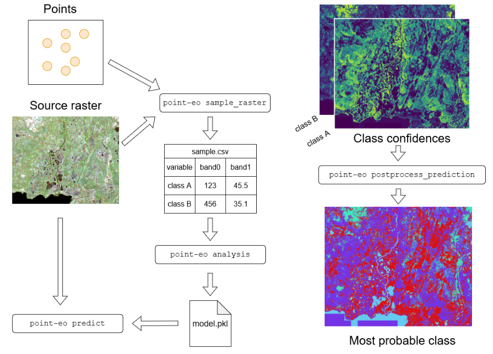
The PointEO is a Python library (scripts) stored locally that were developed internally in SYKE. The purpose of the library is to facilitate the land use prediction using the Random Forest model. By packing the function in a local library it is easier to call them all just when they are needed and makes the process simpler.

The library is given already in the local folder and you just need to run the command sys.path.append() to call available libraries in your home directory.

Feel free to take a look at the Point-EO GitHub Repository.

# adding point-eo from local scripts
home = os.getcwd()
sys.path.append(home)

import point_eo.scripts.sample_xarray as sample_xarray # NOTE: this is my modification to original point-eo repo
import point_eo.scripts.analysis as analysis
import point_eo.scripts.tpot_train as tpot_train
import point_eo.scripts.predict as predict
import point_eo.scripts.postprocess_prediction as postprocess_prediction

We will create an output folder and we will name it basepth

# results folder
if not os.path.exists('output'):
    os.makedirs('output')
    
basepth = os.path.join(home, 'output')

Download Lucas 2018 from Allas

The dataset was stored previously in Allas, the CSC’s cloud storage, and we will download it to our root folder for further use using wget. In case you want to save in a specific folder use the command -P folder_path

!wget -N https://a3s.fi/geoportti_training/lucas2018.tar

--2024-04-08 17:04:47--  https://a3s.fi/geoportti_training/lucas2018.tar
Resolving a3s.fi (a3s.fi)... 86.50.254.19, 86.50.254.18
Connecting to a3s.fi (a3s.fi)|86.50.254.19|:443... connected.
HTTP request sent, awaiting response... 304 Not Modified
File ‘lucas2018.tar’ not modified on server. Omitting download.

Then, we will decompress the datasets in the root folder using the command tar. The command tar unzip previously compressed data and you need to specify the .tar file and the folder where you want to decompress using -C command.

!tar -xf 'lucas2018.tar'

Once you have run the cell you will find the Lucas 2018 data in the subfolder training_data.

The folder contains the data for the whole of Finland and each province.

Let’s take a look at the files and let’s visualize the data at the national level and the selected province we are working on.

# check the files in Lucas 2018 training_data folder
lucas_paths = glob.glob(os.path.join(home, 'training_data/*.shp'))

lucas_files = [path.split('/')[-1] for path in lucas_paths]

print('Files for Lucas 2018 per province:\n')

for file in sorted(lucas_files):

    print('  ', file)

Files for Lucas 2018 per province:

   lucas2018_10_etelasavo.shp
   lucas2018_11_pohjoissavo.shp
   lucas2018_12_pohjoiskarjala.shp
   lucas2018_13_keskisuomi.shp
   lucas2018_14_etelapohjanmaa.shp
   lucas2018_15_pohjanmaa.shp
   lucas2018_16_keskipohjanmaa.shp
   lucas2018_17_pohjoispohjanmaa.shp
   lucas2018_18_kainuu.shp
   lucas2018_19_lappi.shp
   lucas2018_1_uusimaa.shp
   lucas2018_21_ahvenanmaa.shp
   lucas2018_2_varsinaissuomi.shp
   lucas2018_4_satakunta.shp
   lucas2018_5_kantahame.shp
   lucas2018_6_pirkanmaa.shp
   lucas2018_7_paijathame.shp
   lucas2018_8_kymenlaakso.shp
   lucas2018_9_etelakarjala.shp
   lucas_2018.shp

Lucas 2018 in Finland

Let’s give a quick look at national level.

%%time

# Lucas 2018 in Finland
fi_path = os.path.join(home, 'training_data/lucas_2018.shp')
lucas2018_fi = gpd.read_file(fi_path)

CPU times: user 3.44 s, sys: 84 ms, total: 3.52 s
Wall time: 5.33 s

lucas2018_fi.dtypes

OBJECTID         int64
POINT_ID         int64
OFFICE_PI        int64
SURVEYDATE      object
OBS_DIST        object
OBS_DIRECT       int64
OBS_TYPE         int64
LC1             object
LC2             object
LU1             object
LU2             object
LC1_name        object
LU1_name        object
photolinkN      object
photolinkE      object
photolinkS      object
photolinkW      object
photolinkP      object
LCluokka         int64
maakunta_1       int64
geometry      geometry
dtype: object

lucas2018_fi.LU1_name.value_counts()

LU1_name
Forestry                                                 7864
Agriculture                                              3535
Semi-natural and natural areas not in use                2452
Residential                                               711
Road transport                                            698
Amenities, museums, leisure                               224
Mining and quarrying                                      171
Fallow land                                                76
Community services                                         60
Electricity, gas and thermal power distribution            58
Other abandoned areas                                      56
Commerce                                                   38
Railway transport                                          34
Sport                                                      34
Kitchen garden                                             33
Logistics and storage                                      28
Abandoned residential areas                                18
Wood based products                                        15
Air transport                                              14
Construction                                               13
Water transport                                             9
Machinery and equipment                                     6
Abandoned transport areas                                   4
Chemical and allied industries and manufacturing            4
Abandoned industrial areas                                  4
Aquaculture and fishing                                     4
Coal, oil and metal processing                              3
Energy production                                           3
Waste treatment                                             3
Manufacturing of food, beverages and tobacco products       2
Transport via pipelines                                     1
Financial, professional and information services            1
Production of non-metal mineral goods                       1
Telecommunication                                           1
Other primary production                                    1
Printing and reproduction                                   1
Name: count, dtype: int64

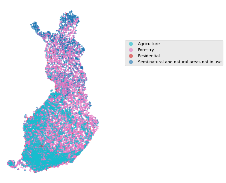
plt.style.use('ggplot')

fig, ax = plt.subplots(figsize=(6, 8))

# set class
class_name = ['Forestry', 'Agriculture', 'Residential', 'Semi-natural and natural areas not in use']
lu_class = lucas2018_fi.loc[lucas2018_fi['LU1_name'].isin(class_name)].sort_values('LU1_name', ascending=False)

# plot
lu_class.plot(ax=ax,
               column='LU1_name', 
               categorical=True, 
               cmap = 'tab10_r',
               markersize= 10,
               alpha = 0.6,
               legend=True,
               legend_kwds={'bbox_to_anchor':(1.2, 0.8)}
              )

plt.axis('off');

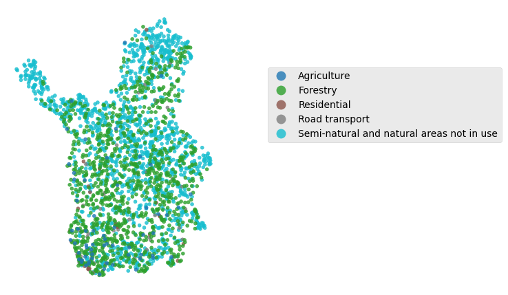
Lucas 2018 in Lapland

We will work in this exercise using the Lapland region.

# get path
lapland_path = os.path.join(home, 'training_data/lucas2018_19_lappi.shp')

# read
lucas2018_lapland = gpd.read_file(lapland_path)

lucas2018_lapland.LU1_name.value_counts()

LU1_name
Semi-natural and natural areas not in use          1333
Forestry                                           1053
Agriculture                                          61
Road transport                                       50
Residential                                          26
Amenities, museums, leisure                          21
Mining and quarrying                                 12
Other abandoned areas                                 9
Community services                                    8
Electricity, gas and thermal power distribution       4
Abandoned transport areas                             4
Fallow land                                           3
Air transport                                         2
Commerce                                              2
Water transport                                       2
Logistics and storage                                 1
Construction                                          1
Wood based products                                   1
Coal, oil and metal processing                        1
Production of non-metal mineral goods                 1
Other primary production                              1
Energy production                                     1
Name: count, dtype: int64

lucas2018_lapland.crs.name

'ETRS89 / TM35FIN(E,N)'

plt.style.use('ggplot')

fig, ax = plt.subplots(figsize=(4, 6))

# set class
class_name = ['Forestry', 'Agriculture', 'Residential', 'Semi-natural and natural areas not in use', 'Road transport',]
lu_class = lucas2018_lapland.loc[lucas2018_lapland['LU1_name'].isin(class_name)].sort_values('LU1_name', ascending=False)

# plot
lu_class.plot(ax=ax,
               column='LU1_name', 
               categorical=True, 
               cmap = 'tab10',
               markersize= 12,
               alpha = 0.8,
               legend=True,
               legend_kwds={'bbox_to_anchor':(1.2, 0.8)}
              )

plt.axis('off');

Download input rasters from Allas

To keep this exercise straightforward we have stored the input raster in Allas. This will make it easy to download and use in the workflow.

You will download a folder input_data that contains:

Filename	Feature	Used in model
ndvi_max_2021_lapland.tif	Normalized Vegetation Index	Yes
km2_lapland.tif	Digital Elevation Model	Yes
tree_classes_lapland.tif	Tree density	Yes
vegetation_height_lapland.tif	Vegetation density	Yes
canopy_cover_lapland.tif	Canopy cover	Yes
s2_nir_lapland.tif	Sentinel 2 Near Infrared	Yes
s2_rgb_lapland.tif	Sentinel 2 bands: red, green, and blue	No
s2_rgb_lapland_band1.tif	Sentinel 2 band blue	Yes
s2_rgb_lapland_band2.tif	Sentinel 2 band green	Yes
s2_rgb_lapland_band3.tif	Sentinel 2 band red	Yes

!wget -N https://a3s.fi/geoportti_training/input_data.tar

--2024-04-08 17:05:02--  https://a3s.fi/geoportti_training/input_data.tar
Resolving a3s.fi (a3s.fi)... 86.50.254.18, 86.50.254.19
Connecting to a3s.fi (a3s.fi)|86.50.254.18|:443... connected.
HTTP request sent, awaiting response... 304 Not Modified
File ‘input_data.tar’ not modified on server. Omitting download.

!tar -xf 'input_data.tar'

Using GeoCubes for downloading data (Optional)

GeoCubes offers raster data for different provinces. You can download datasets using urllib by selecting the region and data from API links in GeoCubes API access.

Attention

If you want to download data from GeoCubes using another Finland province of your interest be aware that sometimes the API might not be working due to maintenance

The next code will help you to download data using API endpoints. It uses a new created folder and urllib.request.urlretrieve()

            # -- Create a results folder
            
            if not os.path.exists('input_data'):
                os.makedirs('input_data')
                
            # -- Function to download from GeoCubes
            
            def download_data(url, output_folder, file_name):
                '''
                Download images from URL to a local path 
                    - params: URL, string
                    - output_folder, string
                    - file_name, string
                '''
                # get url and path
                download_url = url
                out_fn = os.path.join(output_folder, file_name)
                
                print(f"Downloading... {download_url}")
                
                try:
                urllib request
                    r = urllib.request.urlretrieve(download_url, out_fn)
                    
                    print(f"Download completed. Results saved to {out_fn}/n")
            
                except:
            
                    print(f"URL not valid {download_url}\n")
            
            # -- Using function (Example)
            
            url = 'https://vm0160.kaj.pouta.csc.fi/geocubes/clip/10/puustoisuusluokat/maakuntajako:19/202'
            input_data_folder = os.path.join(home, 'input_data')
            file_name = 'tree_classes_lapland.tif'
            
            # run
            download_data(url, input_data_folder, file_name)

Split multi-band rasters to single-band (Optional)

If you have downloaded data from a different province using GeoCubes be aware that RGB images are a composite of Red, Green, and Blue images. As we prefer to have independent data it is recommended to split this multi-band image into single-band images.

For that, you can use the next function in your workflow:

            # -- Function to split a multi-band raster
            
            def split_multiband_raster(input_path, output_folder):
                '''
                Read from local folder a multi-band image and split it single-band
                    - input_path: multi-band tif
                    - output_folder: store single-band tif folder
                '''
                
                # Open the multiband raster
                ds = rxr.open_rasterio(input_path)
            
                # Get the number of bands
                num_bands = ds.shape[0]
            
                # Loop through each band
                for band_index in range(num_bands):
                    
                    # Get the band data
                    band = ds[band_index]
            
                    # Create the output file name
                    output_name = f"multi-band_split_band_{band_index + 1}.tif"
                    output_path = os.path.join(output_folder, output_name)
            
                    # Save the band as a single-band raster
                    band.rio.to_raster(output_path)
            
                    print(f"Band {band_index + 1} saved as {output_path}")
            
             # -- Using function (Example)
            
            input_raster = "input_data/s2_rgb_lapland.tif"
            output_folder = "input_data"
            
            # run
            split_multiband_raster(input_raster, output_folder)

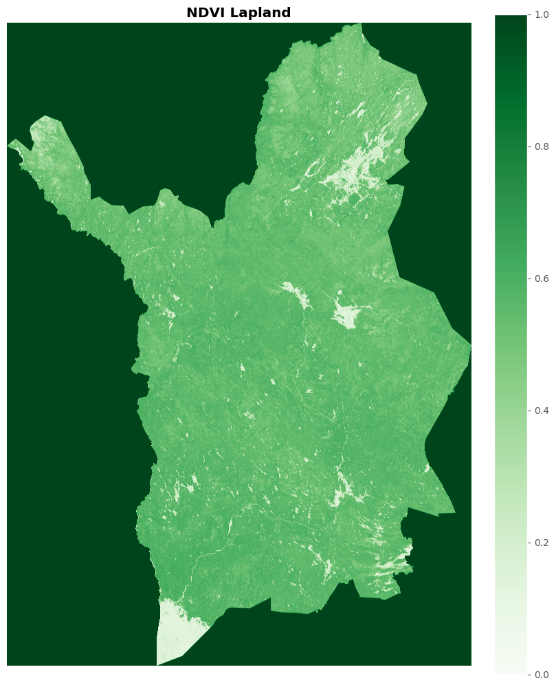
Visualization of input raster - NDVI example

Let’s take a look at the input raster data we are going to use. The library that support raster visualization is rasterio.

# remove the file we are not using
remove_path = glob.glob(os.path.join(home, 'input_data/s2_rgb_lapland.tif'))

# delete not needed file RGB Composition
os.remove(remove_path[0])

# check the files in raster input_data folder
raster_paths = glob.glob(os.path.join(home, 'input_data/*.tif'))

raster_files = [path.split('/')[-1] for path in raster_paths]

print('Files for input raster per variable:\n')

for file in sorted(raster_files):

    print('  ', file)

Files for input raster per variable:

   canopy_cover_lapland.tif
   km2_lapland.tif
   ndvi_max_2021_lapland.tif
   s2_nir_lapland.tif
   s2_rgb_lapland_band1.tif
   s2_rgb_lapland_band2.tif
   s2_rgb_lapland_band3.tif
   tree_classes_lapland.tif
   vegetation_height_lapland.tif

raster_paths

['/projappl/project_2009245/GeoHPC-dev/source/lessons/L3/input_data/canopy_cover_lapland.tif',
 '/projappl/project_2009245/GeoHPC-dev/source/lessons/L3/input_data/ndvi_max_2021_lapland.tif',
 '/projappl/project_2009245/GeoHPC-dev/source/lessons/L3/input_data/vegetation_height_lapland.tif',
 '/projappl/project_2009245/GeoHPC-dev/source/lessons/L3/input_data/s2_rgb_lapland_band1.tif',
 '/projappl/project_2009245/GeoHPC-dev/source/lessons/L3/input_data/s2_rgb_lapland_band3.tif',
 '/projappl/project_2009245/GeoHPC-dev/source/lessons/L3/input_data/s2_nir_lapland.tif',
 '/projappl/project_2009245/GeoHPC-dev/source/lessons/L3/input_data/tree_classes_lapland.tif',
 '/projappl/project_2009245/GeoHPC-dev/source/lessons/L3/input_data/s2_rgb_lapland_band2.tif',
 '/projappl/project_2009245/GeoHPC-dev/source/lessons/L3/input_data/km2_lapland.tif']

fig, ax = plt.subplots(figsize=(8, 10), layout='constrained')

# get path and open
source = 'input_data/ndvi_max_2021_lapland.tif'
img = rasterio.open(source)

# fig
show(img.read(), title='NDVI Lapland', cmap='Greens', ax=ax);

# colorbar
cmap = plt.cm.Greens

fig.colorbar(plt.cm.ScalarMappable(cmap=cmap), 
             ax=ax, 
            )

plt.axis('off');

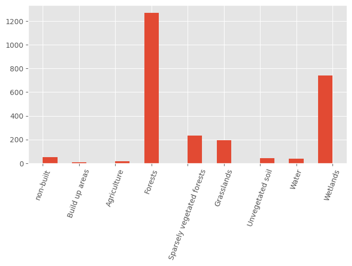
Land Use Class frequency visualization

Let’s take a look at the frequency of Land Use Classes in our selected province. The column we will use is the LCluokka

# Land Use class
lucas2018_lapland.LCluokka.hist(figsize=(8, 4), bins=20)

plt.xticks(ticks = [0, 1, 2, 3, 4, 5, 6, 7, 8],
            labels=['non-built', 'Build up areas', 'Agriculture', 'Forests', 
                    'Sparsely vegetated forests', 'Grasslands',
                    'Unvegetated soil', 'Water', 'Wetlands'],
          rotation=70
          );
    

Create a datacube

A datacube is a structure that keeps many layers of information gathered in a three-dimensional (cubic) form. The x and y axis represents the location of data and every location can store many variables, and the z dimension represents temporal layers. This format is used mainly with environment or Earth Observation data.

We will add our variables to a datacube. Let’s get familiar with the next functions.

def load_raster(raster, band_name):
    '''
    Gives back a raster with an specific band name
    '''
    
    # read
    xds = rxr.open_rasterio(raster)

    name = raster.split('/')[-1].split('.')[0]

    print(f'Loading - {name}')

    return xds.rename(band_name)


def create_cube(input_rasters):
    '''
    Gives back a data cube and a list of band names
    
    NOTE! 
    This function uses delayed functions from Dask
    '''
    
    # Raster input data for sampling
    rasters =  [path for path in input_rasters]
    
    band_names = [name.split('/')[-1].split('.')[0] for name in input_rasters]
    
    # delayed_rasters = [
    #     dask.delayed(load_raster)(raster, band_names[i]) for i, raster in enumerate(rasters)
    #                   ]   
    
    # rasters_to_merge = dask.compute(*delayed_rasters)

    rasters_to_merge = [load_raster(raster, band_names[i]) for i, raster in enumerate(rasters)]

    print(f'Merging...')
    
    cube = xr.merge(rasters_to_merge)

    print(f'Transposing...')
    
    cube = cube.transpose('band', 'y', 'x')

    print(f'Done!')
    
    return cube, band_names

raster_paths

['/projappl/project_2009245/GeoHPC-dev/source/lessons/L3/input_data/canopy_cover_lapland.tif',
 '/projappl/project_2009245/GeoHPC-dev/source/lessons/L3/input_data/ndvi_max_2021_lapland.tif',
 '/projappl/project_2009245/GeoHPC-dev/source/lessons/L3/input_data/vegetation_height_lapland.tif',
 '/projappl/project_2009245/GeoHPC-dev/source/lessons/L3/input_data/s2_rgb_lapland_band1.tif',
 '/projappl/project_2009245/GeoHPC-dev/source/lessons/L3/input_data/s2_rgb_lapland_band3.tif',
 '/projappl/project_2009245/GeoHPC-dev/source/lessons/L3/input_data/s2_nir_lapland.tif',
 '/projappl/project_2009245/GeoHPC-dev/source/lessons/L3/input_data/tree_classes_lapland.tif',
 '/projappl/project_2009245/GeoHPC-dev/source/lessons/L3/input_data/s2_rgb_lapland_band2.tif',
 '/projappl/project_2009245/GeoHPC-dev/source/lessons/L3/input_data/km2_lapland.tif']

%%time

cube, band_names = create_cube(raster_paths)

Loading - canopy_cover_lapland
Loading - ndvi_max_2021_lapland
Loading - vegetation_height_lapland
Loading - s2_rgb_lapland_band1
Loading - s2_rgb_lapland_band3
Loading - s2_nir_lapland
Loading - tree_classes_lapland
Loading - s2_rgb_lapland_band2
Loading - km2_lapland
Merging...
Transposing...
Done!
CPU times: user 191 ms, sys: 48.9 ms, total: 240 ms
Wall time: 2.28 s

cube

<xarray.Dataset> Size: 33GB
Dimensions:                    (band: 1, x: 38477, y: 53241)
Coordinates:
  * band                       (band) int64 8B 1
  * x                          (x) float64 308kB 2.431e+05 ... 6.279e+05
  * y                          (y) float64 426kB 7.776e+06 ... 7.244e+06
    spatial_ref                int64 8B 0
Data variables:
    canopy_cover_lapland       (band, y, x) uint8 2GB ...
    ndvi_max_2021_lapland      (band, y, x) uint8 2GB ...
    vegetation_height_lapland  (band, y, x) uint8 2GB ...
    s2_rgb_lapland_band1       (band, y, x) uint16 4GB ...
    s2_rgb_lapland_band3       (band, y, x) uint16 4GB ...
    s2_nir_lapland             (band, y, x) uint16 4GB ...
    tree_classes_lapland       (band, y, x) uint8 2GB ...
    s2_rgb_lapland_band2       (band, y, x) uint16 4GB ...
    km2_lapland                (band, y, x) float32 8GB ...
Attributes:
    AREA_OR_POINT:  Area
    _FillValue:     127
    scale_factor:   1.0
    add_offset:     0.0

xarray.Dataset

• Dimensions:
  • band: 1
  • x: 38477
  • y: 53241
• Coordinates: (4)
  • band
    (band)
    int64
    1

    array([1])

  • x
    (x)
    float64
    2.431e+05 2.431e+05 ... 6.279e+05

    array([243095.91, 243105.91, 243115.91, ..., 627835.91, 627845.91, 627855.91])

  • y
    (y)
    float64
    7.776e+06 7.776e+06 ... 7.244e+06

    array([7776445.217, 7776435.217, 7776425.217, ..., 7244065.217, 7244055.217,
           7244045.217])

  • spatial_ref
    ()
    int64
    0

    crs_wkt :

    PROJCS["ETRS89 / TM35FIN(E,N)",GEOGCS["ETRS89",DATUM["European_Terrestrial_Reference_System_1989",SPHEROID["GRS 1980",6378137,298.257222101,AUTHORITY["EPSG","7019"]],AUTHORITY["EPSG","6258"]],PRIMEM["Greenwich",0,AUTHORITY["EPSG","8901"]],UNIT["degree",0.0174532925199433,AUTHORITY["EPSG","9122"]],AUTHORITY["EPSG","4258"]],PROJECTION["Transverse_Mercator"],PARAMETER["latitude_of_origin",0],PARAMETER["central_meridian",27],PARAMETER["scale_factor",0.9996],PARAMETER["false_easting",500000],PARAMETER["false_northing",0],UNIT["metre",1,AUTHORITY["EPSG","9001"]],AXIS["Easting",EAST],AXIS["Northing",NORTH],AUTHORITY["EPSG","3067"]]

    semi_major_axis :

    6378137.0

    semi_minor_axis :

    6356752.314140356

    inverse_flattening :

    298.257222101

    reference_ellipsoid_name :

    GRS 1980

    longitude_of_prime_meridian :

    0.0

    prime_meridian_name :

    Greenwich

    geographic_crs_name :

    ETRS89

    horizontal_datum_name :

    European Terrestrial Reference System 1989

    projected_crs_name :

    ETRS89 / TM35FIN(E,N)

    grid_mapping_name :

    transverse_mercator

    latitude_of_projection_origin :

    0.0

    longitude_of_central_meridian :

    27.0

    false_easting :

    500000.0

    false_northing :

    0.0

    scale_factor_at_central_meridian :

    0.9996

    spatial_ref :

    PROJCS["ETRS89 / TM35FIN(E,N)",GEOGCS["ETRS89",DATUM["European_Terrestrial_Reference_System_1989",SPHEROID["GRS 1980",6378137,298.257222101,AUTHORITY["EPSG","7019"]],AUTHORITY["EPSG","6258"]],PRIMEM["Greenwich",0,AUTHORITY["EPSG","8901"]],UNIT["degree",0.0174532925199433,AUTHORITY["EPSG","9122"]],AUTHORITY["EPSG","4258"]],PROJECTION["Transverse_Mercator"],PARAMETER["latitude_of_origin",0],PARAMETER["central_meridian",27],PARAMETER["scale_factor",0.9996],PARAMETER["false_easting",500000],PARAMETER["false_northing",0],UNIT["metre",1,AUTHORITY["EPSG","9001"]],AXIS["Easting",EAST],AXIS["Northing",NORTH],AUTHORITY["EPSG","3067"]]

    GeoTransform :

    243090.91 10.0 0.0 7776450.217 0.0 -10.0

    array(0)

• Data variables: (9)
  • canopy_cover_lapland
    (band, y, x)
    uint8
    ...

    AREA_OR_POINT :

    Area

    _FillValue :

    127

    scale_factor :

    1.0

    add_offset :

    0.0

    [2048553957 values with dtype=uint8]

  • ndvi_max_2021_lapland
    (band, y, x)
    uint8
    ...

    AREA_OR_POINT :

    Area

    _FillValue :

    255

    scale_factor :

    1.0

    add_offset :

    0.0

    [2048553957 values with dtype=uint8]

  • vegetation_height_lapland
    (band, y, x)
    uint8
    ...

    AREA_OR_POINT :

    Area

    STATISTICS_APPROXIMATE :

    YES

    STATISTICS_MAXIMUM :

    231

    STATISTICS_MEAN :

    33.499432741694

    STATISTICS_MINIMUM :

    0

    STATISTICS_STDDEV :

    33.902745917398

    STATISTICS_VALID_PERCENT :

    38.93

    _FillValue :

    255

    scale_factor :

    1.0

    add_offset :

    0.0

    [2048553957 values with dtype=uint8]

  • s2_rgb_lapland_band1
    (band, y, x)
    uint16
    ...

    AREA_OR_POINT :

    Area

    _FillValue :

    65535

    scale_factor :

    1.0

    add_offset :

    0.0

    [2048553957 values with dtype=uint16]

  • s2_rgb_lapland_band3
    (band, y, x)
    uint16
    ...

    AREA_OR_POINT :

    Area

    _FillValue :

    65535

    scale_factor :

    1.0

    add_offset :

    0.0

    [2048553957 values with dtype=uint16]

  • s2_nir_lapland
    (band, y, x)
    uint16
    ...

    AREA_OR_POINT :

    Area

    _FillValue :

    65535

    scale_factor :

    1.0

    add_offset :

    0.0

    [2048553957 values with dtype=uint16]

  • tree_classes_lapland
    (band, y, x)
    uint8
    ...

    AREA_OR_POINT :

    Area

    _FillValue :

    127

    scale_factor :

    1.0

    add_offset :

    0.0

    [2048553957 values with dtype=uint8]

  • s2_rgb_lapland_band2
    (band, y, x)
    uint16
    ...

    AREA_OR_POINT :

    Area

    _FillValue :

    65535

    scale_factor :

    1.0

    add_offset :

    0.0

    [2048553957 values with dtype=uint16]

  • km2_lapland
    (band, y, x)
    float32
    ...

    AREA_OR_POINT :

    Area

    _FillValue :

    -9999.0

    scale_factor :

    1.0

    add_offset :

    0.0

    [2048553957 values with dtype=float32]

• Indexes: (3)
  • band
    PandasIndex

    PandasIndex(Index([1], dtype='int64', name='band'))

  • x
    PandasIndex

    PandasIndex(Index([243095.91, 243105.91, 243115.91, 243125.91, 243135.91, 243145.91,
           243155.91, 243165.91, 243175.91, 243185.91,
           ...
           627765.91, 627775.91, 627785.91, 627795.91, 627805.91, 627815.91,
           627825.91, 627835.91, 627845.91, 627855.91],
          dtype='float64', name='x', length=38477))

  • y
    PandasIndex

    PandasIndex(Index([7776445.217, 7776435.217, 7776425.217, 7776415.217, 7776405.217,
           7776395.217, 7776385.217, 7776375.217, 7776365.217, 7776355.217,
           ...
           7244135.217, 7244125.217, 7244115.217, 7244105.217, 7244095.217,
           7244085.217, 7244075.217, 7244065.217, 7244055.217, 7244045.217],
          dtype='float64', name='y', length=53241))

• Attributes: (4)

  AREA_OR_POINT :

  Area

  _FillValue :

  127

  scale_factor :

  1.0

  add_offset :

  0.0

Store bands for point-eo sampling script

We will keep the band names in a band_names.txt file for further use in our model.

band_name_file = os.path.join(basepth, 'band_names.txt')

with open(band_name_file, 'w') as fp:
    
    for item in band_names:
        
        fp.write("%s\n" % item)

Sample raster using point-eo for sampling

In this process we are going to sample the raster data we have using the Lucas 2018 dataset. To use the point-eo tool we will use a parsing library called argparse that creates inputs variables while using scripts in terminal.

Follow the next process using the sample_xarray function from point-eo tool.

%%time

# -- paths
input_shape = os.path.join(home, 'training_data/lucas2018_19_lappi.shp')
output_sample_folder = os.path.join(basepth,'sampled')

# --  initiate parsing
parser = argparse.ArgumentParser()
subparsers = parser.add_subparsers(title="Available commands", dest="script")

# -- choose sampling xarrat - data cube
sample_xarray.add_args(subparsers)

# -- arguments
args = parser.parse_args(['sample_raster',
                            '--input', input_shape,
                            '--input_raster', 'dummy_placeholder',
                            '--target', 'LCluokka',
                            '--band_names', band_name_file,
                            '--out_folder', output_sample_folder])

# -- set input_raster to xarray variable - Data Cube
args.input_raster = cube

# -- RUN
sample_xarray.main(args)

Sampling xarray dataset using points from /projappl/project_2009245/GeoHPC-dev/source/lessons/L3/training_data/lucas2018_19_lappi.shp
Using bandnames:
['canopy_cover_lapland',
 'ndvi_max_2021_lapland',
 'vegetation_height_lapland',
 's2_rgb_lapland_band1',
 's2_rgb_lapland_band3',
 's2_nir_lapland',
 'tree_classes_lapland',
 's2_rgb_lapland_band2',
 'km2_lapland']
Saved outputs to /projappl/project_2009245/GeoHPC-dev/source/lessons/L3/output/sampled/xarray__lucas2018_19_lappi__LCluokka.csv
CPU times: user 35.2 s, sys: 25.9 s, total: 1min 1s
Wall time: 3min 13s

# read sampling file
path = os.path.join(basepth,'sampled', 'xarray__lucas2018_19_lappi__LCluokka.csv')

df = pd.read_csv(path)

df.head()

	LCluokka	canopy_cover_lapland	ndvi_max_2021_lapland	vegetation_height_lapland	s2_rgb_lapland_band1	s2_rgb_lapland_band3	s2_nir_lapland	tree_classes_lapland	s2_rgb_lapland_band2	km2_lapland
0	6	127.0	112.0	255.0	1047.0	841.0	1500.0	30.0	977.0	859.72390
1	6	127.0	113.0	255.0	1135.0	995.0	1510.0	30.0	1103.0	778.58010
2	5	127.0	142.0	255.0	743.0	600.0	2150.0	30.0	730.0	699.85986
3	3	15.0	178.0	4.0	224.0	271.0	3281.0	11.0	423.0	197.96394
4	3	2.0	167.0	3.0	267.0	311.0	2159.0	11.0	429.0	151.15020

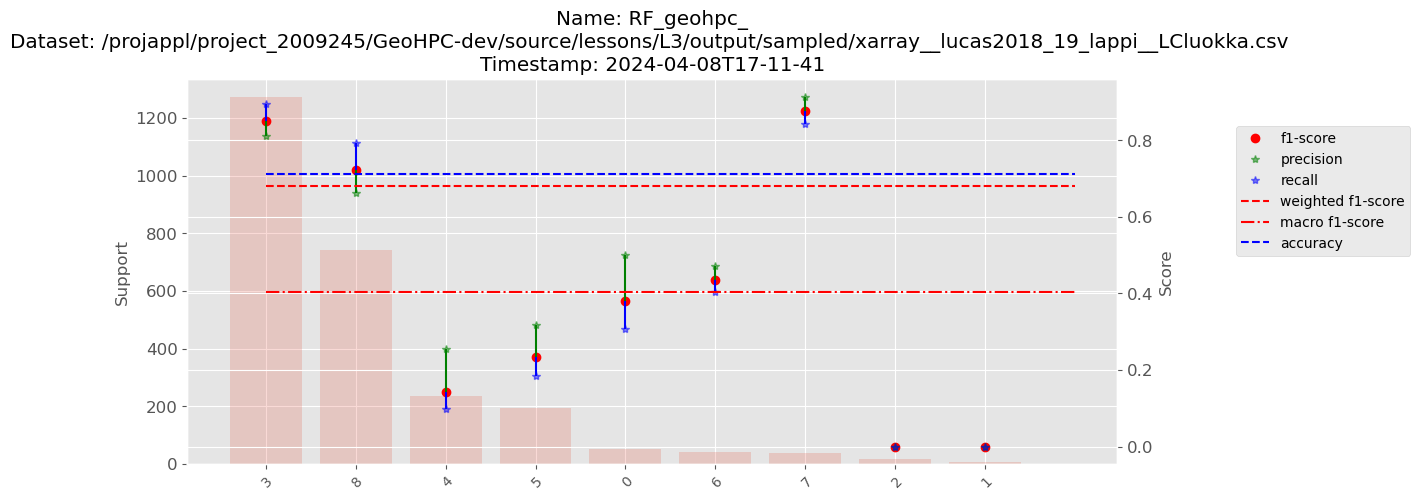
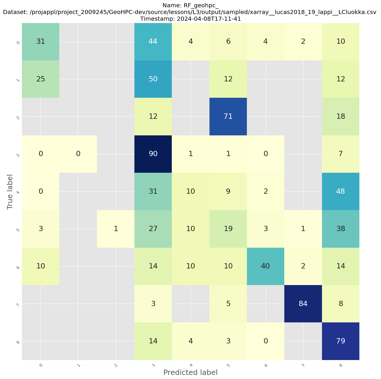
Training with Random Forest model

Let’s continue training our model using Random Forest implemented in point-eo tool.

#  Training, analysis with the defaults (Random Forest)

# -- paths
input_sampling_file = os.path.join(basepth,'sampled','xarray__lucas2018_19_lappi__LCluokka.csv')
rf_folder = os.path.join(basepth,'model_fitting_RF')


# -- start parser
parser = argparse.ArgumentParser()
subparsers = parser.add_subparsers(title="Available commands", dest="script")
analysis.add_args(subparsers)

# -- arguments
args = parser.parse_args(['analysis',
                            '--input', input_sampling_file,
                            '--out_folder', rf_folder,
                            '--out_prefix', 'RF_geohpc_',
                            '--decimal', '.',
                            '--separator',','])

# -- RUN
analysis.main(args)

Input csv: /projappl/project_2009245/GeoHPC-dev/source/lessons/L3/output/sampled/xarray__lucas2018_19_lappi__LCluokka.csv
Model: RF


### Data info ###

Columns. First one is chosen as target
Index		Column
0		LCluokka
1		canopy_cover_lapland
2		ndvi_max_2021_lapland
3		vegetation_height_lapland
4		s2_rgb_lapland_band1
5		s2_rgb_lapland_band3
6		s2_nir_lapland
7		tree_classes_lapland
8		s2_rgb_lapland_band2
9		km2_lapland


Shape of data table:
rows: 2598
columns: 10

Target class distribution
label	count
LCluokka
3    1271
8     741
4     235
5     194
0      52
6      42
7      38
2      17
1       8
Name: count, dtype: int64




### Starting cross-validation ###

Random forest parameters:
{'bootstrap': True, 'ccp_alpha': 0.0, 'class_weight': None, 'criterion': 'gini', 'max_depth': None, 'max_features': 'sqrt', 'max_leaf_nodes': None, 'max_samples': None, 'min_impurity_decrease': 0.0, 'min_samples_leaf': 1, 'min_samples_split': 2, 'min_weight_fraction_leaf': 0.0, 'monotonic_cst': None, 'n_estimators': 100, 'n_jobs': -1, 'oob_score': False, 'random_state': None, 'verbose': 0, 'warm_start': False}

Fold 0:
Accuracy: 0.721
Precision: 0.680
F1: 0.692

Fold 1:
Accuracy: 0.688
Precision: 0.632
F1: 0.652

Fold 2:
Accuracy: 0.723
Precision: 0.682
F1: 0.693

Fold 3:
Accuracy: 0.711
Precision: 0.661
F1: 0.679

Fold 4:
Accuracy: 0.717
Precision: 0.667
F1: 0.682

Overall results:
Accuracy: 0.712
Precision: 0.664
F1: 0.680

Using categorical units to plot a list of strings that are all parsable as floats or dates. If these strings should be plotted as numbers, cast to the appropriate data type before plotting.
Using categorical units to plot a list of strings that are all parsable as floats or dates. If these strings should be plotted as numbers, cast to the appropriate data type before plotting.
Using categorical units to plot a list of strings that are all parsable as floats or dates. If these strings should be plotted as numbers, cast to the appropriate data type before plotting.
Using categorical units to plot a list of strings that are all parsable as floats or dates. If these strings should be plotted as numbers, cast to the appropriate data type before plotting.
Using categorical units to plot a list of strings that are all parsable as floats or dates. If these strings should be plotted as numbers, cast to the appropriate data type before plotting.
Using categorical units to plot a list of strings that are all parsable as floats or dates. If these strings should be plotted as numbers, cast to the appropriate data type before plotting.
              precision    recall  f1-score   support

           0       0.50      0.31      0.38        52
           1       0.00      0.00      0.00         8
           2       0.00      0.00      0.00        17
           3       0.81      0.90      0.85      1271
           4       0.26      0.10      0.14       235
           5       0.32      0.19      0.23       194
           6       0.47      0.40      0.44        42
           7       0.91      0.84      0.88        38
           8       0.66      0.79      0.72       741

    accuracy                           0.71      2598
   macro avg       0.44      0.39      0.40      2598
weighted avg       0.66      0.71      0.68      2598

Saved classification graph to /projappl/project_2009245/GeoHPC-dev/source/lessons/L3/output/model_fitting_RF/RF_geohpc___xarray__lucas2018_19_lappi__LCluokka__2024-04-08T17-11-41_metrics.png

Saved confusion matrix to /projappl/project_2009245/GeoHPC-dev/source/lessons/L3/output/model_fitting_RF/RF_geohpc___xarray__lucas2018_19_lappi__LCluokka__2024-04-08T17-11-41_confusion.png

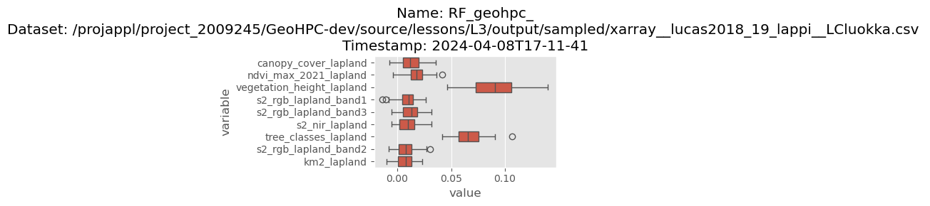
Saved permutation importance to /projappl/project_2009245/GeoHPC-dev/source/lessons/L3/output/model_fitting_RF/RF_geohpc___xarray__lucas2018_19_lappi__LCluokka__2024-04-08T17-11-41_permutation_importance.png
Saved model to /projappl/project_2009245/GeoHPC-dev/source/lessons/L3/output/model_fitting_RF/RF_geohpc___xarray__lucas2018_19_lappi__LCluokka__2024-04-08T17-11-41_model.pkl

Parallelization of Random Forest

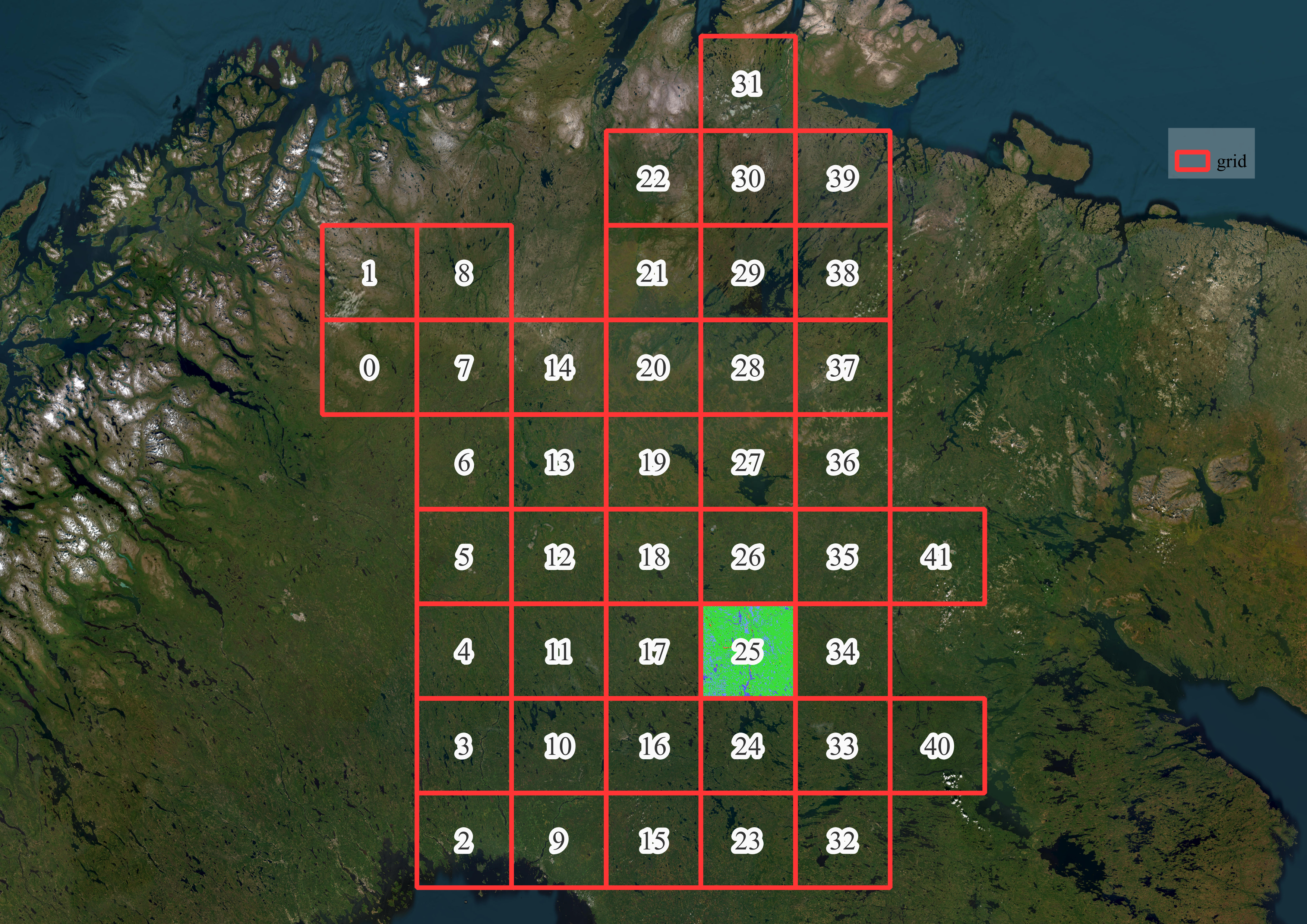
Grid creation

We have a quite large area of the province so we are going to create grids that allow us to parallelize the process using each square. Follow step by step about the grid creation and the Land Use Class prediction with Random Forest.

Get familiar with the next function.

def create_grid(study_area, grid_size_m):
    '''
    Give back a Geodataframe with specific grid size based on study area
        study_area: geodaframe. default point geometry. crs not geographic
        grid_size_m: size of grid side in meters

        return: Geodataframe of polygons. Grid
    '''
    print(f'CRS of study area: {study_area.crs.name}')
    
    # get bounds of province
    xmin, ymin, xmax, ymax = study_area.buffer(100).total_bounds

    # grid size
    length = grid_size_m
    wide = grid_size_m

    cols = list(np.arange(xmin, xmax + wide, wide))
    rows = list(np.arange(ymin, ymax + length, length))

    polygons = []
    for x in cols[:-1]:
        for y in rows[:-1]:
            polygons.append(Polygon([(x,y), (x+wide, y), (x+wide, y+length), (x, y+length)]))
    
    grid = gpd.GeoDataFrame({'geometry':polygons}, crs = study_area.crs)

    # ----- Remove empty grids

    index_true = []
    
    for row in grid.itertuples():

        # check if contains
        contains = study_area.intersects(row.geometry)
  
        if True in contains.unique():

            # catch index of grid that contains study area
            index_true.append(row.Index)

    # subset only valid grids
    grid_valid = grid.loc[grid.index.isin(index_true)]

    # reset index
    grid_valid = grid_valid.reset_index(drop=True)
    
    print(f'Total grids: {len(grid_valid)}')
    
    return grid_valid

# create grids
grid = create_grid(lucas2018_lapland, 60000)

CRS of study area: ETRS89 / TM35FIN(E,N)
Total grids: 42

# save grid
grid.to_file('output/grid.gpkg')

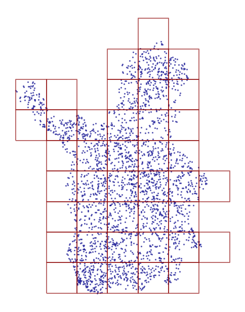
plt.style.use('ggplot')

fig, ax = plt.subplots(figsize=(6, 8))

# plot
lucas2018_lapland.plot(ax=ax,
                       color='darkblue',
                       markersize= 3,
                       alpha = 0.6,
                      )

grid.plot(ax=ax,
          facecolor="none", 
          edgecolor="darkred",
          linewidth=1.4,
          alpha=0.6
         )

plt.axis('off');

Automating Inference with Random Forest PointEO

We are going to pack the inference of Random Forest per area. The next function will use as input the fitted model, the independent grid, and some paths for results.

Note

We added a couple of lines in the function that remove intermediate files. We do it to save memory in the disk.

def run_random_forest(data_cube, grid_square, grid_index, output_folder = basepth):
    '''
    Run random forest using default PointEO parameters with Grid squares
        data_cube: data cube with input raster of the whole study area
        grid_square: geom 
        grid_index: n index of the grid for model prediction
    '''
    grid_index = '00'+ str(grid_index)
    grid_index = grid_index[-2:]

    # -- default filepaths

    # paths: model, predict folder
    
    model_path = glob.glob(os.path.join(basepth, f'model_fitting_RF', f'RF*LCluokka*{date.today()}*_model.pkl'))[0]
    print(f'Model: {model_path}')
    
    predict_folder = os.path.join(basepth, f'predict_output_RF_{grid_index}')
    resolution_file = os.path.join(basepth, f"out_RF_{grid_index}.vrt")
    postprocess_folder = os.path.join(basepth, f'land_use_results_RF')
    
    result_path = os.path.join(basepth, f'preprocess_RF_Grid-{grid_index}.tif')

    # --------------------------

    # --> if exists omit the grid cell

    ms_result = os.path.join(postprocess_folder, f'out_RF_{grid_index}_S.tif')
    
    if not os.path.exists(ms_result):
        
        # get bounds of grid
        xmin = grid_square.bounds[0]
        ymin = grid_square.bounds[1]
        xmax = grid_square.bounds[2]
        ymax = grid_square.bounds[3]
        
        # subset data cube
        Fx = cube.where((xmin < cube.x) 
                        & (cube.x < xmax)
                        & (ymin < cube.y) 
                        & (cube.y < ymax), drop=True).to_array().squeeze()
    
        # cell size of the interference blocks
        grid_cells = predict.create_cell_grid(Fx, 10000)
        
        # load rf-model from the analysis stem
        with open(model_path, "rb") as f:
            RF_model = pickle.load(f)
    
        # ----- predict Random Forest
    
        
        predict.calculate(model = RF_model,
                          Fx = Fx,
                          cell_list = grid_cells,
                          verbose=2,
                          out_folder = predict_folder)
    
        # combine blocks
        predict.merge_folder(predict_folder, resolution_file)
    
        # save as geotiff
        Rx = rxr.open_rasterio(
                                resolution_file,
                                chunks={"band": -1, "x": 2**10, "y": 2**10},
                                lock=False,
                                parallel=True,
                            )
    
        # save as tif
        Rx.rio.to_raster(result_path)
    
        # ----- Postprocess prediction
    
        # initiate parser
        parser = argparse.ArgumentParser()
        subparsers = parser.add_subparsers(title="Available commands", dest="script")
        postprocess_prediction.add_args(subparsers)
    
        # arguments
        args = parser.parse_args(['postprocess_prediction',
                                    '--input_raster', resolution_file,
                                    '--out_folder', postprocess_folder
                                    ])
    
        # run
        postprocess_prediction.main(args)

        # ---------------------------------------------------------- remove intermediate info for saving memory

        # folders
        folders = glob.glob(os.path.join(output_folder, '*output*'))
        
        for folder in folders:
        
            shutil.rmtree(folder)
        
        # files
        files = glob.glob(os.path.join(output_folder, '*.vrt'))
        
        for file in files:
        
            os.remove(file)

        pre_files = glob.glob(os.path.join(output_folder, 'preprocess*.tif'))
    
        for pre_file in pre_files:
    
            os.remove(pre_file)

    else:

        print(f'processed {ms_result}')

Single grid square test

Let’s check the model using only a single grid square from our grid.

s = time.time()

# test function with 1 grid square

grid_index = 1

# get geom
geom_grid = grid.at[grid_index, 'geometry']

# Run RF
run_random_forest(cube, geom_grid, grid_index);

single_time = time.time() - s

Model: /projappl/project_2009245/GeoHPC-dev/source/lessons/L3/output/model_fitting_RF/RF_geohpc___xarray__lucas2018_19_lappi__LCluokka__2024-04-08T14-22-12_model.pkl
processed /projappl/project_2009245/GeoHPC-dev/source/lessons/L3/output/land_use_results_RF/out_RF_01_S.tif

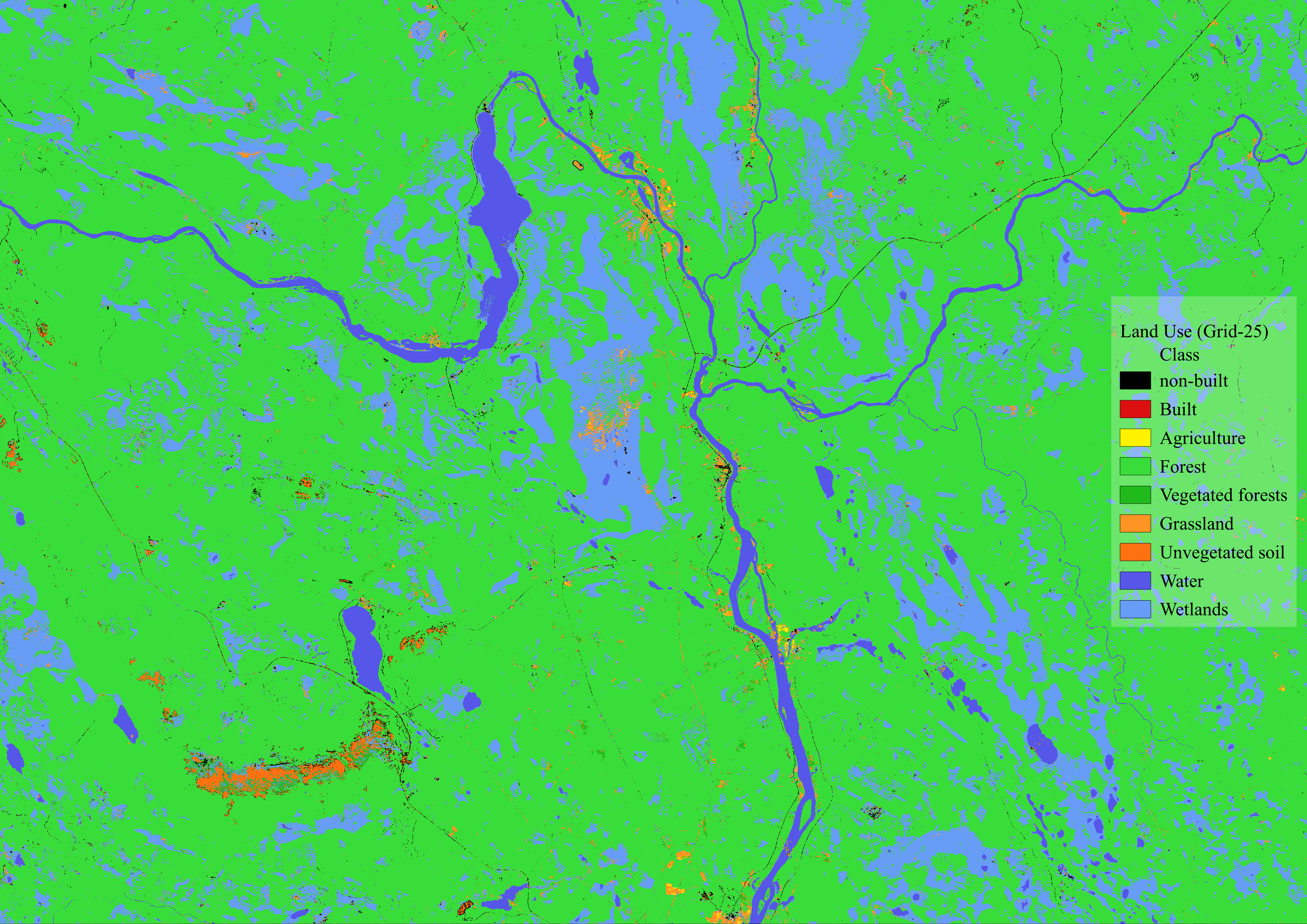
Land Use prediction visualization

The results will be found in the postprocess_folder that we named land_use_results_RF. The file that contains the suffix _S is the one that contains the predicted land use. In this case the file is out_RF_25_S.tif

Let’s check briefly the results for the Grid-25

Create a Dask Client

To use the computational resources in Parallel we need to create a Dask Cluster using the Client function. You can read a bit more in the Dask Documentation. There is an extension for Jupyter Lab called dask-labextension that we installed in our environment. You will find a Dask logo in the left options bar of Jupyter Lab that will allow you to create a Cluster. Simply, click on the + NEW cluster, and then click on < > to add the client to the cell.

Note

You need to delete the code in the cell below and add a new client tcp. Like in Figure 1.

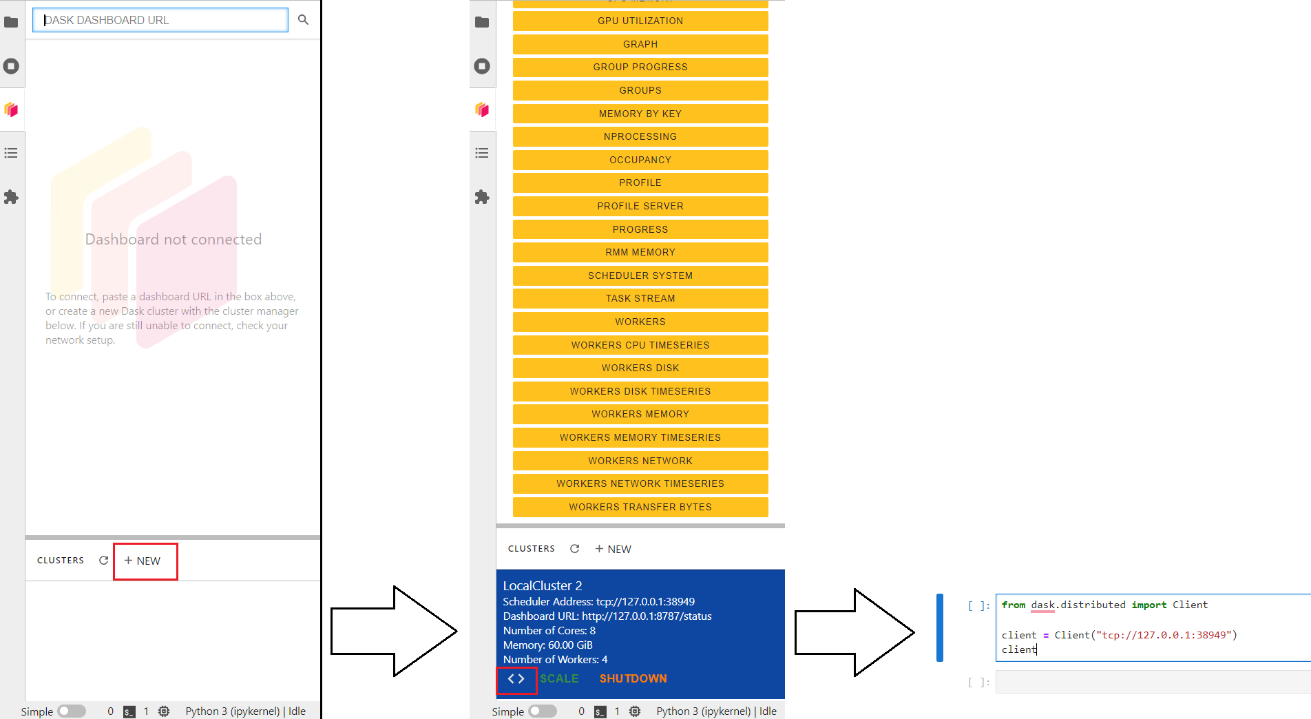
Feel free to Launch dashboard in Jupyter Lab to see the performance of the supercomputer.

from dask.distributed import Client

client = Client("tcp://127.0.0.1:37379")
client

Client

Client-16d2f008-f5b2-11ee-a55f-ac1f6bb239f0

Connection method: Direct
Dashboard: http://127.0.0.1:8787/status

Launch dashboard in JupyterLab

Scheduler Info

Scheduler

Scheduler-75a8662b-7085-42dc-9637-8774587bdda6

Comm: tcp://127.0.0.1:37379	Workers: 4
Dashboard: http://127.0.0.1:8787/status	Total threads: 8
Started: Just now	Total memory: 32.00 GiB

Workers

Worker: 0

Comm: tcp://127.0.0.1:35675	Total threads: 2
Dashboard: http://127.0.0.1:36423/status	Memory: 8.00 GiB
Nanny: tcp://127.0.0.1:33259
Local directory: /run/nvme/job_21127759/tmp/dask-scratch-space/worker-luvc5oke
Tasks executing:	Tasks in memory:
Tasks ready:	Tasks in flight:
CPU usage: 2.0%	Last seen: Just now
Memory usage: 136.39 MiB	Spilled bytes: 0 B
Read bytes: 10.20 kiB	Write bytes: 9.54 kiB

Worker: 1

Comm: tcp://127.0.0.1:45239	Total threads: 2
Dashboard: http://127.0.0.1:36173/status	Memory: 8.00 GiB
Nanny: tcp://127.0.0.1:46161
Local directory: /run/nvme/job_21127759/tmp/dask-scratch-space/worker-ofjrg1a1
Tasks executing:	Tasks in memory:
Tasks ready:	Tasks in flight:
CPU usage: 2.0%	Last seen: Just now
Memory usage: 137.73 MiB	Spilled bytes: 0 B
Read bytes: 9.85 kiB	Write bytes: 9.19 kiB

Worker: 2

Comm: tcp://127.0.0.1:40011	Total threads: 2
Dashboard: http://127.0.0.1:34795/status	Memory: 8.00 GiB
Nanny: tcp://127.0.0.1:34085
Local directory: /run/nvme/job_21127759/tmp/dask-scratch-space/worker-p28zfw34
Tasks executing:	Tasks in memory:
Tasks ready:	Tasks in flight:
CPU usage: 2.0%	Last seen: Just now
Memory usage: 137.26 MiB	Spilled bytes: 0 B
Read bytes: 9.88 kiB	Write bytes: 9.22 kiB

Worker: 3

Comm: tcp://127.0.0.1:45167	Total threads: 2
Dashboard: http://127.0.0.1:34653/status	Memory: 8.00 GiB
Nanny: tcp://127.0.0.1:40351
Local directory: /run/nvme/job_21127759/tmp/dask-scratch-space/worker-4v7hbxse
Tasks executing:	Tasks in memory:
Tasks ready:	Tasks in flight:
CPU usage: 2.0%	Last seen: Just now
Memory usage: 137.09 MiB	Spilled bytes: 0 B
Read bytes: 8.61 kiB	Write bytes: 7.94 kiB

Delayed functions

In Dask you can parallelize custom algorithms using the dask.delayed function. Not everything can fit in a Dask object so in this case the parallelization is sent as a function to the scheduler or cluster.

We will use delayed functions for each grid square.

grid.head()

	geometry
0	POLYGON ((249631.084 7580490.936, 309631.084 7...
1	POLYGON ((249631.084 7640490.936, 309631.084 7...
2	POLYGON ((309631.084 7280490.936, 369631.084 7...
3	POLYGON ((309631.084 7340490.936, 369631.084 7...
4	POLYGON ((309631.084 7400490.936, 369631.084 7...

%%time

# create a list of delayed objects
delayed_RF_functions = [dask.delayed((run_random_forest)(cube, geom, i)) 
                        for i, geom in grid.itertuples()]

# run
with ProgressBar():
    dask.compute(delayed_RF_functions)

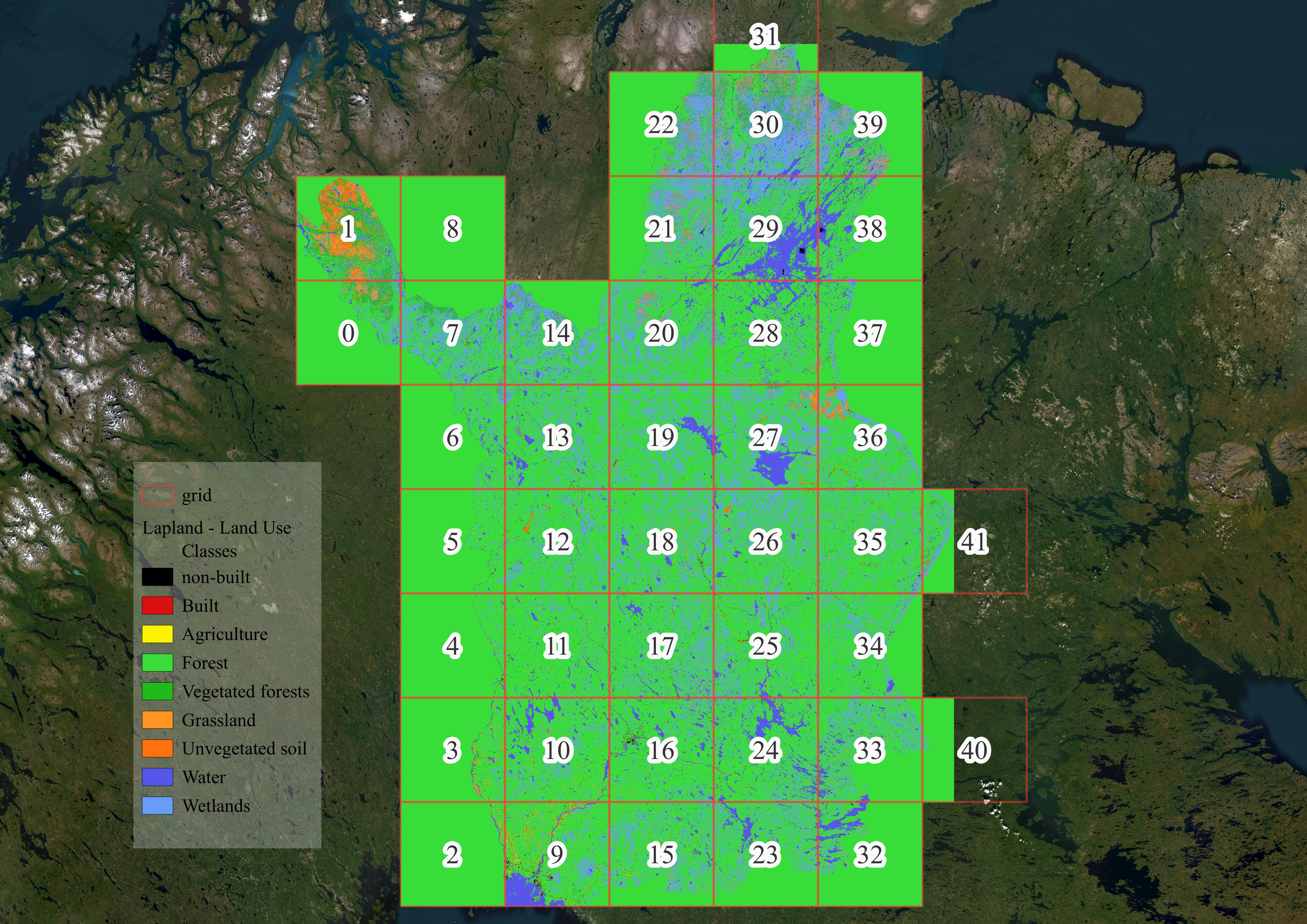
Visualization of the final result

Let’s look at the final map of our province. Remember the results are stored in the folder land_use_results_RF in the files specified with index and S key like: out_RF_<index>_S.tif.

land_use_results = glob.glob(os.path.join(basepth, 'land_use_results_RF', 'out*_S.tif'))

land_use_results

['/projappl/project_2009245/GeoHPC-dev/source/lessons/L3/output/land_use_results_RF/out_RF_25_S.tif',
 '/projappl/project_2009245/GeoHPC-dev/source/lessons/L3/output/land_use_results_RF/out_RF_02_S.tif',
 '/projappl/project_2009245/GeoHPC-dev/source/lessons/L3/output/land_use_results_RF/out_RF_39_S.tif',
 '/projappl/project_2009245/GeoHPC-dev/source/lessons/L3/output/land_use_results_RF/out_RF_17_S.tif',
 '/projappl/project_2009245/GeoHPC-dev/source/lessons/L3/output/land_use_results_RF/out_RF_28_S.tif',
 '/projappl/project_2009245/GeoHPC-dev/source/lessons/L3/output/land_use_results_RF/out_RF_15_S.tif',
 '/projappl/project_2009245/GeoHPC-dev/source/lessons/L3/output/land_use_results_RF/out_RF_10_S.tif',
 '/projappl/project_2009245/GeoHPC-dev/source/lessons/L3/output/land_use_results_RF/out_RF_08_S.tif',
 '/projappl/project_2009245/GeoHPC-dev/source/lessons/L3/output/land_use_results_RF/out_RF_12_S.tif',
 '/projappl/project_2009245/GeoHPC-dev/source/lessons/L3/output/land_use_results_RF/out_RF_18_S.tif',
 '/projappl/project_2009245/GeoHPC-dev/source/lessons/L3/output/land_use_results_RF/out_RF_11_S.tif',
 '/projappl/project_2009245/GeoHPC-dev/source/lessons/L3/output/land_use_results_RF/out_RF_00_S.tif',
 '/projappl/project_2009245/GeoHPC-dev/source/lessons/L3/output/land_use_results_RF/out_RF_13_S.tif',
 '/projappl/project_2009245/GeoHPC-dev/source/lessons/L3/output/land_use_results_RF/out_RF_21_S.tif',
 '/projappl/project_2009245/GeoHPC-dev/source/lessons/L3/output/land_use_results_RF/out_RF_01_S.tif',
 '/projappl/project_2009245/GeoHPC-dev/source/lessons/L3/output/land_use_results_RF/out_RF_14_S.tif',
 '/projappl/project_2009245/GeoHPC-dev/source/lessons/L3/output/land_use_results_RF/out_RF_23_S.tif',
 '/projappl/project_2009245/GeoHPC-dev/source/lessons/L3/output/land_use_results_RF/out_RF_20_S.tif',
 '/projappl/project_2009245/GeoHPC-dev/source/lessons/L3/output/land_use_results_RF/out_RF_36_S.tif',
 '/projappl/project_2009245/GeoHPC-dev/source/lessons/L3/output/land_use_results_RF/out_RF_34_S.tif',
 '/projappl/project_2009245/GeoHPC-dev/source/lessons/L3/output/land_use_results_RF/out_RF_27_S.tif',
 '/projappl/project_2009245/GeoHPC-dev/source/lessons/L3/output/land_use_results_RF/out_RF_29_S.tif',
 '/projappl/project_2009245/GeoHPC-dev/source/lessons/L3/output/land_use_results_RF/out_RF_16_S.tif',
 '/projappl/project_2009245/GeoHPC-dev/source/lessons/L3/output/land_use_results_RF/out_RF_40_S.tif',
 '/projappl/project_2009245/GeoHPC-dev/source/lessons/L3/output/land_use_results_RF/out_RF_06_S.tif',
 '/projappl/project_2009245/GeoHPC-dev/source/lessons/L3/output/land_use_results_RF/out_RF_26_S.tif',
 '/projappl/project_2009245/GeoHPC-dev/source/lessons/L3/output/land_use_results_RF/out_RF_31_S.tif',
 '/projappl/project_2009245/GeoHPC-dev/source/lessons/L3/output/land_use_results_RF/out_RF_24_S.tif',
 '/projappl/project_2009245/GeoHPC-dev/source/lessons/L3/output/land_use_results_RF/out_RF_03_S.tif',
 '/projappl/project_2009245/GeoHPC-dev/source/lessons/L3/output/land_use_results_RF/out_RF_09_S.tif',
 '/projappl/project_2009245/GeoHPC-dev/source/lessons/L3/output/land_use_results_RF/out_RF_05_S.tif',
 '/projappl/project_2009245/GeoHPC-dev/source/lessons/L3/output/land_use_results_RF/out_RF_22_S.tif',
 '/projappl/project_2009245/GeoHPC-dev/source/lessons/L3/output/land_use_results_RF/out_RF_32_S.tif',
 '/projappl/project_2009245/GeoHPC-dev/source/lessons/L3/output/land_use_results_RF/out_RF_33_S.tif',
 '/projappl/project_2009245/GeoHPC-dev/source/lessons/L3/output/land_use_results_RF/out_RF_37_S.tif',
 '/projappl/project_2009245/GeoHPC-dev/source/lessons/L3/output/land_use_results_RF/out_RF_35_S.tif',
 '/projappl/project_2009245/GeoHPC-dev/source/lessons/L3/output/land_use_results_RF/out_RF_38_S.tif',
 '/projappl/project_2009245/GeoHPC-dev/source/lessons/L3/output/land_use_results_RF/out_RF_30_S.tif',
 '/projappl/project_2009245/GeoHPC-dev/source/lessons/L3/output/land_use_results_RF/out_RF_07_S.tif',
 '/projappl/project_2009245/GeoHPC-dev/source/lessons/L3/output/land_use_results_RF/out_RF_41_S.tif',
 '/projappl/project_2009245/GeoHPC-dev/source/lessons/L3/output/land_use_results_RF/out_RF_19_S.tif',
 '/projappl/project_2009245/GeoHPC-dev/source/lessons/L3/output/land_use_results_RF/out_RF_04_S.tif']

Let’s check the last results in QGIS